In this chapter, we explore different methods used in the literature to recalibrate a model. The basic idea is to learn a function \(g(\cdot)\) mapping scores \(s(x)\) into probability estimates \(g(p) := \mathbb{E}[D \mid s(x) = p]\). To avoid overfitting the training data while learning that mapping, we will rely on data from the calibration set.
As in Chapter 1, we will transform the true probabilities \(p\) of simulated data and consider these transformed values \(p^u\) to be scores that could be returned by a classifier model.
Display the definitions of colors.
library(tidyverse)
── Attaching core tidyverse packages ──────────────────────── tidyverse 2.0.0 ──
✔ dplyr     1.1.4     ✔ readr     2.1.5
✔ forcats   1.0.0     ✔ stringr   1.5.1
✔ ggplot2   3.5.1     ✔ tibble    3.2.1
✔ lubridate 1.9.3     ✔ tidyr     1.3.1
✔ purrr     1.0.2
── Conflicts ────────────────────────────────────────── tidyverse_conflicts() ──
✖ dplyr::filter() masks stats::filter()
✖ dplyr::lag()    masks stats::lag()
ℹ Use the conflicted package (<http://conflicted.r-lib.org/>) to force all conflicts to become errors
We use the same DGP as that presented in Section 1.1 in Chapter 1. Let us redefine here the function which simulates data.
#' Simulates data#'#' @param n_obs number of desired observations#' @param seed seed to use to generate the data#' @param alpha scale parameter for the latent probability (if different #' from 1, the probabilities are transformed and it may induce decalibration)#' @param gamma scale parameter for the latent score (if different from 1, #' the probabilities are transformed and it may induce decalibration)sim_data <-function(n_obs =2000, seed, alpha =1, gamma =1) {set.seed(seed) x1 <-runif(n_obs) x2 <-runif(n_obs) x3 <-runif(n_obs) x4 <-runif(n_obs) epsilon_p <-rnorm(n_obs, mean =0, sd = .5)# True latent score eta <--0.1*x1 +0.05*x2 +0.2*x3 -0.05*x4 + epsilon_p# Transformed latent score eta_u <- gamma * eta# True probability p <- (1/ (1+exp(-eta)))# Transformed probability p_u <- ((1/ (1+exp(-eta_u))))^alpha# Observed event d <-rbinom(n_obs, size =1, prob = p)tibble(# Event Probabilityp = p,p_u = p_u,# Binary outcome variabled = d,# Variablesx1 = x1,x2 = x2,x3 = x3,x4 = x4 )}
2.2 Recalibration Methods
To compare different calibration metrics, we will split our dataset into the following sets:
a calibration set: to train the recalibrator
a test set: on which we will compute the calibration metrics.
Note
In the general case where the scores are obtained using a classifier, the dataset needs to be split into three parts instead of two:
a train set: to train the classifier
a calibration set: to train the recalibrator
a test set: on which we will compute the calibration metrics.
We define (as in the previous chapter 1) a function to create the splits.
#' Get calibration/test samples from the DGP#'#' @param seed seed to use to generate the data#' @param n_obs number of desired observations#' @param alpha scale parameter for the latent probability (if different #' from 1, the probabilities are transformed and it may induce decalibration)#' @param gamma scale parameter for the latent score (if different from 1, #' the probabilities are transformed and it may induce decalibration)get_samples <-function(seed,n_obs =2000,alpha =1,gamma =1) {set.seed(seed) data_all <-sim_data(n_obs = n_obs, seed = seed, alpha = alpha, gamma = gamma )# Calibration/test sets---- data <- data_all |>select(d, x1:x4) probas <- data_all |>select(p) calib_index <-sample(1:nrow(data), size = .6*nrow(data), replace =FALSE) tb_calib <- data |>slice(calib_index) tb_test <- data |>slice(-calib_index) probas_calib <- probas |>slice(calib_index) probas_test <- probas |>slice(-calib_index)list(data_all = data_all,data = data,tb_calib = tb_calib,tb_test = tb_test,probas_calib = probas_calib,probas_test = probas_test,calib_index = calib_index,seed = seed,n_obs = n_obs,alpha = alpha,gamma = gamma )}
We simulate a single toy dataset to begin with. Simulations made on replications will be done later.
Let us consider a case where the probabilities are distorted using \(\alpha=.25\).
Platt scaling (Platt et al. 1999) consists of applying logistic regression to \((d,s(x))\) where \(d\) denotes the binary outcome and \(s(x)\) is the vector of predicted scores.
# Logistic regressionlr <-glm(d ~ p_u, family =binomial(link ='logit'), data = data_all_calib)
The predicted values in the calibration set and in the test set:
score_c_platt_calib <-predict(lr, newdata = data_all_calib, type ="response")score_c_platt_test <-predict(lr, newdata = data_all_test, type ="response")
Let us create a vector of values to estimate the calibration curve.
linspace <-seq(0, 1, length.out =100)
We can then use the fitted logistic regression to make predictions on this vector of values:
score_c_platt_linspace <-predict( lr, newdata =tibble(p_u = linspace), type ="response")
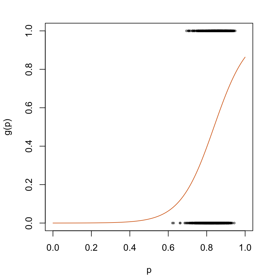
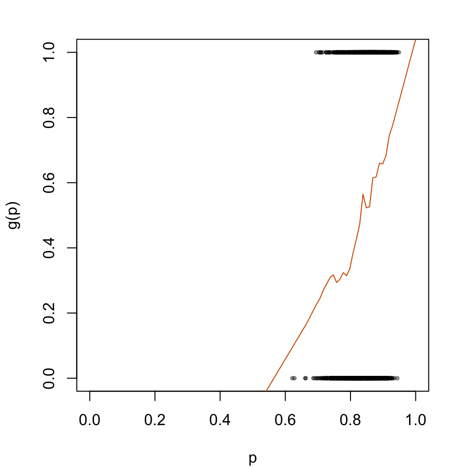
The predicted probabilities \(p_u\) will then be transformed according to the logistic model depicted in Figure 5.1.
par(mar =c(4.1, 4.1, 2.1, 2.1))plot( data_all_calib$p_u, data_all_calib$d, type ="p", cex = .5, pch =19,col =adjustcolor("black", alpha.f = .4),xlab ="p", ylab ="g(p)",xlim =c(0,1))lines(x = tb_scores_c_platt$linspace, y = tb_scores_c_platt$p_c, type ="l", col ="#D55E00")
Figure 2.1: Recalibration Using Platt Scaling
2.2.2 Isotonic Regression
Isotonic regression is a non parametric approach using the pool-adjacent-violators (PAV) algorithm, introduced by Zadrozny and Elkan (2002). In a nutshell, it assumes that the predicted scores of the initial model (random forest in this notebook) reproduces well the ranks of the observations. Under this assumption, the mapping \(g(\cdot)\) from the scores \(s(x)\) into the probabilities \(g(p)\) is non-decreasing. It is then possible to use isotonic regression to learn the mapping. The PAV algorithm works as follows:
At a given iteration: consider the ranked examples \(x_{i-1}\) and \(x_{i}\).
If the current values of the function to be learned is such that \(g(x_{i-1}) \leq g(x_{i})\), nothing changes.
Otherwise, \(x_1\) and \(x_2\) are called pair-adjacent violators. The values of \(g(x_{i-1})\) and \(g(x_{i})\) are replaced by their mean \((g(x_{i-1}) + g(x_{i})) / 2\). If this move creates earlier violations (\(g(x_{i-1})\) might be lower than \(g(x_{i-2})\)), a new value is set for \(g(x_{i-2})\), \(g(x_{i-1})\), and \(g(x_{i})\), as the average in the group.
Let us compute the isototic least squares regression on the scores \(p_u\):
iso <-isoreg(x = data_all_calib$p_u, y = data_all_calib$d)
Transforming the fit into a function:
fit_iso <-as.stepfun(iso)
The predicted values on the calibration set and on the test set:
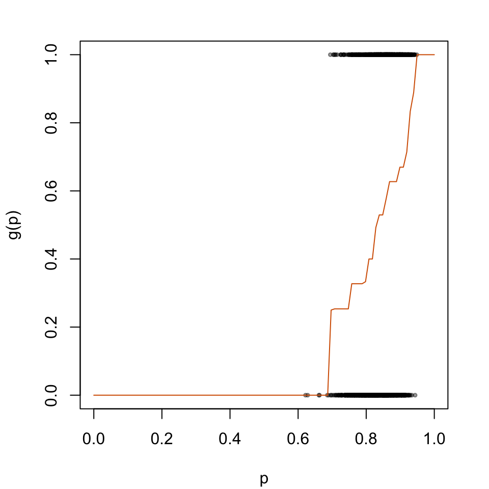
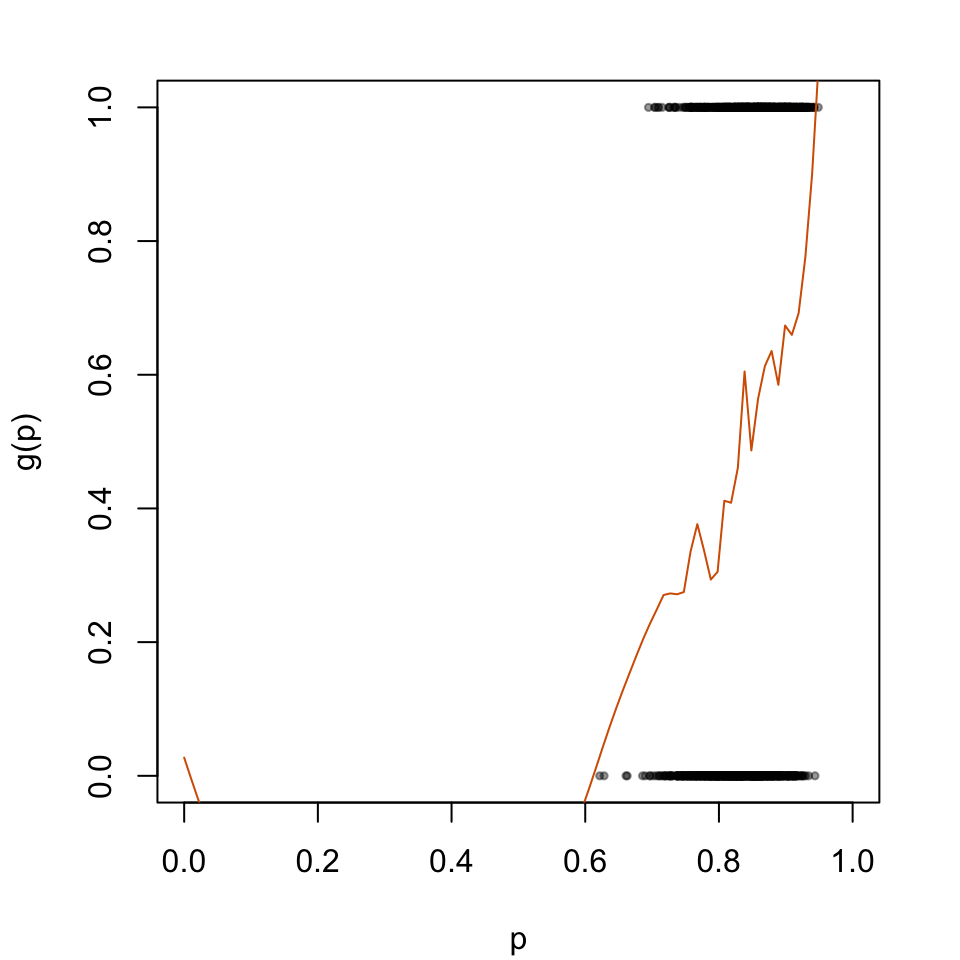
The predicted probabilities \(p_u\) will then be transformed according to the logistic model depicted in Figure 5.2.
par(mar =c(4.1, 4.1, 2.1, 2.1))plot( data_all_calib$p_u, data_all_calib$d, type ="p", cex = .5, pch =19,col =adjustcolor("black", alpha.f = .4),xlab ="p", ylab ="g(p)",xlim =c(0, 1))lines(x = tb_scores_c_isotonic$linspace, y = tb_scores_c_isotonic$p_c, type ="l", col ="#D55E00")
Figure 2.2: Recalibration Using Isotonic Regression
2.2.3 Beta Calibration
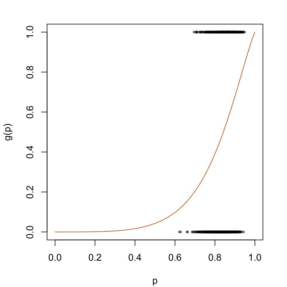
Instead of fitting a logistic regression on the predicted values, as we know that the distribution of the values are bounded to \([0,1]\), it is possible to use beta calibration Kull, Silva Filho, and Flach (2017). With this method, instead of assuming that the scores obtained by the classifier are normally distributed (as is the underlying assumption when using Platt scaling), the scores are assumed to follow a Beta distribution. We estimate : \[\mu(s;a,b,c) = \frac{1}{1 + \frac{1}{e^c \frac{s^a}{(1-s)^b}}}\]
library(betacal)# Beta calibration using the paper packagebc <-beta_calibration(p = data_all_calib$p_u, y = data_all_calib$d, parameters ="abm"# 3 parameters a, b & m)
[1] -126.7104
[1] 42.94288
The predicted values on the calibration set and on the test set:
The predicted probabilities \(p_u\) will then be transformed according to the logistic model depicted in Figure 5.3
par(mar =c(4.1, 4.1, 2.1, 2.1))plot( data_all_calib$p_u, data_all_calib$d, type ="p", cex = .5, pch =19,col =adjustcolor("black", alpha.f = .4),xlab ="p", ylab ="g(p)",xlim =c(0, 1))lines(x = tb_scores_c_beta$linspace, y = tb_scores_c_beta$p_c, type ="l", col ="#D55E00")
Figure 2.3: Recalibration Using Beta Calibration
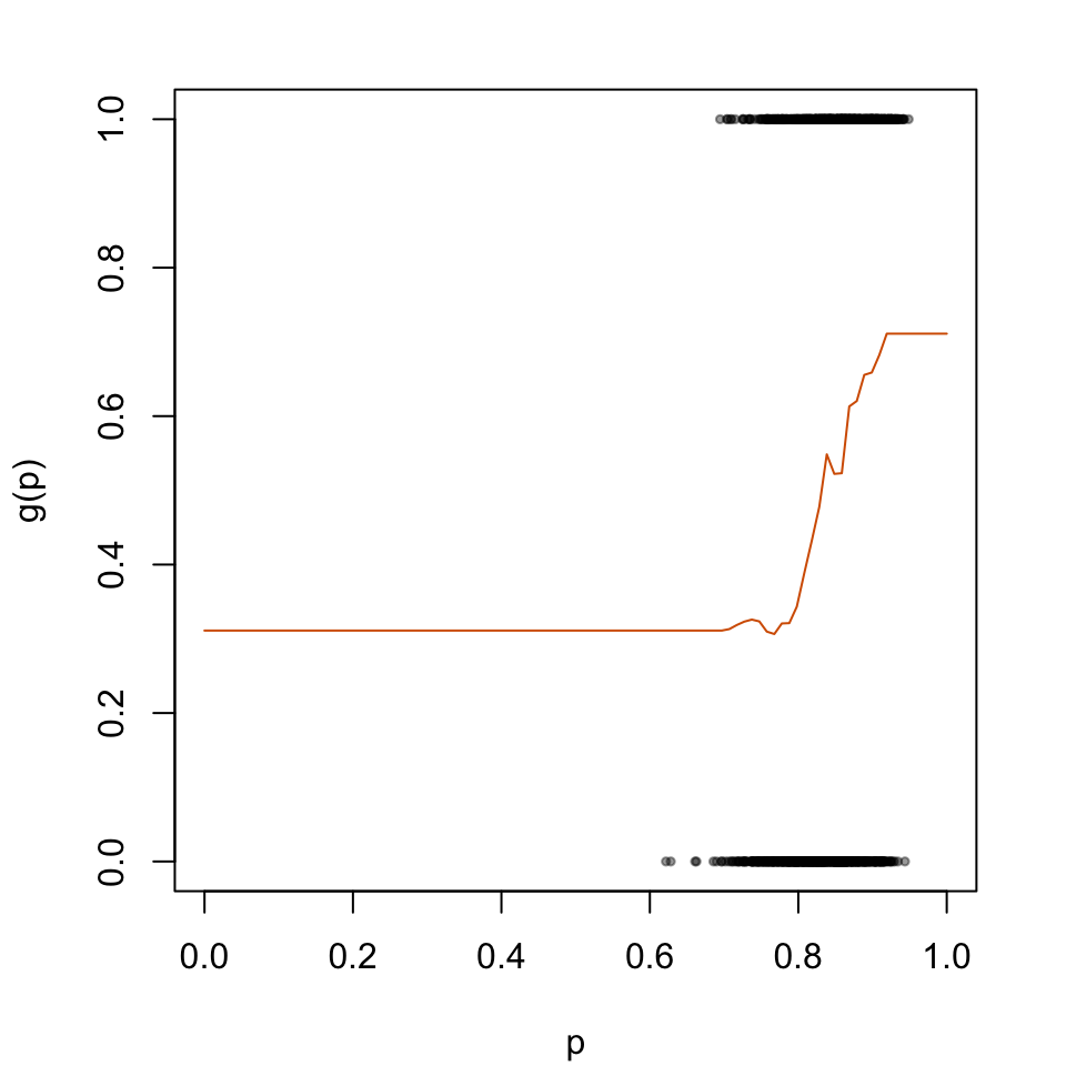
2.2.4 Local Regression
Local regression fits polynomials locally to each bin defined by nn argument of the locfit() function.
library(locfit)
locfit 1.5-9.9 2024-03-01
Attaching package: 'locfit'
The following object is masked from 'package:purrr':

    none
We consider three versions here, with different degrees for the polynomials (0, 1, or 2). We set the number of nearest neighbors to use to nn =0.15, that is, 15%.
e_calib_error() to compute the Expected Calibration Error (see Section 1.2.1.3 in Chapter 1). This function relies on get_summary_bins() which computes summary statistics for binomial observed data and predicted scores returned by a model.
Display the functions used to compute the ECE
#' Computes summary statistics for binomial observed data and predicted scores#' returned by a model#'#' @param obs vector of observed events#' @param scores vector of predicted probabilities#' @param k number of classes to create (quantiles, default to `10`)#' @param threshold classification threshold (default to `.5`)#' @return a tibble where each row correspond to a bin, and each columns are:#' - `score_class`: level of the decile that the bin represents#' - `nb`: number of observation#' - `mean_obs`: average of obs (proportion of positive events)#' - `mean_score`: average predicted score (confidence)#' - `sum_obs`: number of positive events (number of positive events)#' - `accuracy`: accuracy (share of correctly predicted, using the#' threshold)get_summary_bins <-function(obs, scores,k =10, threshold = .5) { breaks <-quantile(scores, probs = (0:k) / k) tb_breaks <-tibble(breaks = breaks, labels =0:k) |>group_by(breaks) |>slice_tail(n =1) |>ungroup() x_with_class <-tibble(obs = obs,score = scores, ) |>mutate(score_class =cut( score,breaks = tb_breaks$breaks,labels = tb_breaks$labels[-1],include.lowest =TRUE ),pred_class =ifelse(score > threshold, 1, 0),correct_pred = obs == pred_class ) x_with_class |>group_by(score_class) |>summarise(nb =n(),mean_obs =mean(obs),mean_score =mean(score), # confidencesum_obs =sum(obs),accuracy =mean(correct_pred) ) |>ungroup() |>mutate(score_class =as.character(score_class) |>as.numeric() ) |>arrange(score_class)}#' Expected Calibration Error#'#' @param obs vector of observed events#' @param scores vector of predicted probabilities#' @param k number of classes to create (quantiles, default to `10`)#' @param threshold classification threshold (default to `.5`)e_calib_error <-function(obs, scores, k =10, threshold = .5) { summary_bins <-get_summary_bins(obs = obs, scores = scores, k = k, threshold = .5 ) summary_bins |>mutate(ece_bin = nb *abs(accuracy - mean_score)) |>summarise(ece =1/sum(nb) *sum(ece_bin)) |>pull(ece)}
qmse_error() to compute Quantile-based MSE (see Section 1.2.1.4 in Chapter 1). This function also relies on get_summary_bins().
Display the functions used to compute the QMSE
#' Quantile-Based MSE#'#' @param obs vector of observed events#' @param scores vector of predicted probabilities#' @param k number of classes to create (quantiles, default to `10`)#' @param threshold classification threshold (default to `.5`)qmse_error <-function(obs, scores, k =10, threshold = .5) { summary_bins <-get_summary_bins(obs = obs, scores = scores, k = k, threshold = .5 ) summary_bins |>mutate(qmse_bin = nb * (mean_obs - mean_score)^2) |>summarise(qmse =1/sum(nb) *sum(qmse_bin)) |>pull(qmse)}
wmse_error() to compute Weighted MSE (see Section 1.2.1.5 in Chapter 1). This function relies on local_ci_scores() which identifies the nearest neighbors of a certain predicted score and then calculates the mean scores in that neighborhood accompanied with its confidence interval.
Display the functions used to compute the WMSE
#' @param obs vector of observed events#' @param scores vector of predicted probabilities#' @param tau value at which to compute the confidence interval#' @param nn fraction of nearest neighbors#' @param prob level of the confidence interval (default to `.95`)#' @param method Which method to use to construct the interval. Any combination#' of c("exact", "ac", "asymptotic", "wilson", "prop.test", "bayes", "logit",#' "cloglog", "probit") is allowed. Default is "all".#' @return a tibble with a single row that corresponds to estimations made in#' the neighborhood of a probability $p=\tau$`, using the fraction `nn` of#' neighbors, where the columns are:#' - `score`: score tau in the neighborhood of which statistics are computed#' - `mean`: estimation of $E(d | s(x) = \tau)$#' - `lower`: lower bound of the confidence interval#' - `upper`: upper bound of the confidence intervallocal_ci_scores <-function(obs, scores, tau, nn,prob = .95,method ="probit") {# Identify the k nearest neighbors based on hat{p} k <-round(length(scores) * nn) rgs <-rank(abs(scores - tau), ties.method ="first") idx <-which(rgs <= k)binom.confint(x =sum(obs[idx]),n =length(idx),conf.level = prob,methods = method )[, c("mean", "lower", "upper")] |>tibble() |>mutate(xlim = tau) |>relocate(xlim, .before = mean)}#' Compute the Weighted Mean Squared Error to assess the calibration of a model#'#' @param local_scores tibble with expected scores obtained with the #' `local_ci_scores()` function#' @param scores vector of raw predicted probabilitiesweighted_mse <-function(local_scores, scores) {# To account for border bias (support is [0,1]) scores_reflected <-c(-scores, scores, 2- scores) dens <-density(x = scores_reflected, from =0, to =1, n =length(local_scores$xlim) )# The weights weights <- dens$y local_scores |>mutate(wmse_p = (xlim - mean)^2,weight =!!weights ) |>summarise(wmse =sum(weight * wmse_p) /sum(weight)) |>pull(wmse)}
#' Calibration score using Local Regression#' #' @param obs vector of observed events#' @param scores vector of predicted probabilitieslocal_calib_score <-function(obs, scores) {# Add a little noise to the scores, to avoir crashing R scores <- scores +rnorm(length(scores), 0, .001) locfit_0 <-locfit(formula = d ~lp(scores, nn =0.15, deg =0), kern ="rect", maxk =200, data =tibble(d = obs,scores = scores ) )# Predictions on [0,1] linspace_raw <-seq(0, 1, length.out =100)# Restricting this space to the range of observed scores keep_linspace <-which(linspace_raw >=min(scores) & linspace_raw <=max(scores)) linspace <- linspace_raw[keep_linspace] locfit_0_linspace <-predict(locfit_0, newdata = linspace) locfit_0_linspace[locfit_0_linspace >1] <-1 locfit_0_linspace[locfit_0_linspace <0] <-0# Squared difference between predicted value and the bissector, weighted by the density of values scores_reflected <-c(-scores, scores, 2- scores) dens <-density(x = scores_reflected, from =0, to =1, n =length(linspace_raw) )# The weights weights <- dens$y[keep_linspace]weighted.mean((linspace - locfit_0_linspace)^2, weights)}
Then, we define the recalibrate() function which recalibrate a model using the observed events \(d\), the predicted associated probabilities \(p^u\) and a given recalibration technique (as presented above in Section 2.2).
#' Recalibrates scores using a calibration#' #' @param obs_calib vector of observed events in the calibration set#' @param scores_calib vector of predicted probabilities in the calibration set#' #' @param obs_test vector of observed events in the test set#' @param scores_test vector of predicted probabilities in the test set#' @param method recalibration method (`"platt"` for Platt-Scaling, #' `"isotonic"` for isotonic regression, `"beta"` for beta calibration, #' `"locfit"` for local regression)#' @param iso_params list of named parameters to use in the local regression #' (`nn` for fraction of nearest neighbors to use, `deg` for degree)#' @param linspace vector of alues at which to compute the recalibrated scores#' @returns list of three elements: recalibrated scores on the calibration set,#' recalibrated scores on the test set, and recalibrated scores on a segment #' of valuesrecalibrate <-function(obs_calib, scores_calib, obs_test, scores_test,method =c("platt", "isotonic", "beta", "locfit"),iso_params =NULL,linspace =NULL) {if (is.null(linspace)) linspace <-seq(0, 1, length.out =100) data_calib <-tibble(d = obs_calib, p_u = scores_calib) data_test <-tibble(d = obs_test, p_u = scores_test)if (method =="platt") { lr <-glm(d ~ p_u, family =binomial(link ='logit'), data = data_calib)# Recalibrated scores on calibration and test set score_c_calib <-predict(lr, newdata = data_calib, type ="response") score_c_test <-predict(lr, newdata = data_test, type ="response")# Recalibrated values along a segment score_c_linspace <-predict( lr, newdata =tibble(p_u = linspace), type ="response" ) } elseif (method =="isotonic") { iso <-isoreg(x = data_calib$p_u, y = data_calib$d) fit_iso <-as.stepfun(iso)# Recalibrated scores on calibration and test set score_c_calib <-fit_iso(data_calib$p_u) score_c_test <-fit_iso(data_test$p_u)# Recalibrated values along a segment score_c_linspace <-fit_iso(linspace) } elseif (method =="beta") {capture.output({ bc <-beta_calibration(p = data_calib$p_u, y = data_calib$d, parameters ="abm"# 3 parameters a, b & m ) })# Recalibrated scores on calibration and test set score_c_calib <-beta_predict(p = data_calib$p_u, bc) score_c_test <-beta_predict(p = data_test$p_u, bc)# Recalibrated values along a segment score_c_linspace <-beta_predict(linspace, bc) } elseif (method =="locfit") {# Deg 0 locfit_reg <-locfit(formula = d ~lp(p_u, nn = iso_params$nn, deg = iso_params$deg), kern ="rect", maxk =200, data = data_calib )# Recalibrated scores on calibration and test set score_c_calib <-predict(locfit_reg, newdata = data_calib) score_c_calib[score_c_calib <0] <-0 score_c_calib[score_c_calib >1] <-1 score_c_test <-predict(locfit_reg, newdata = data_test) score_c_test[score_c_test <0] <-0 score_c_test[score_c_test >1] <-1# Recalibrated values along a segment score_c_linspace <-predict(locfit_reg, newdata = linspace) score_c_linspace[score_c_linspace <0] <-0 score_c_linspace[score_c_linspace >1] <-1 } else {stop(str_c('Wrong method. Use one of the following:','"platt", "isotonic", "beta", "locfit"' )) }# Format results in tibbles:# For calibration set tb_score_c_calib <-tibble(d = obs_calib,p_u = scores_calib,p_c = score_c_calib )# For test set tb_score_c_test <-tibble(d = obs_test,p_u = scores_test,p_c = score_c_test )# For linear space tb_score_c_linspace <-tibble(linspace = linspace,p_c = score_c_linspace )list(tb_score_c_calib = tb_score_c_calib,tb_score_c_test = tb_score_c_test,tb_score_c_linspace = tb_score_c_linspace )}
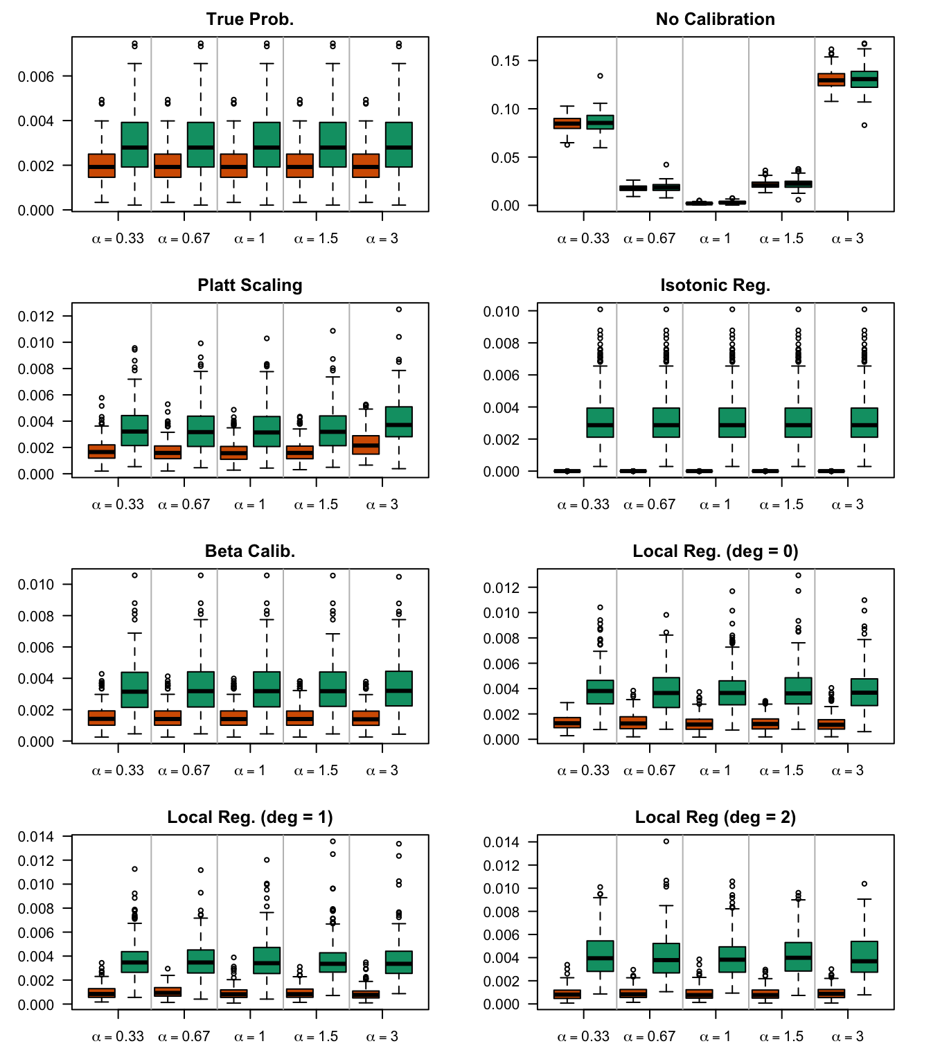
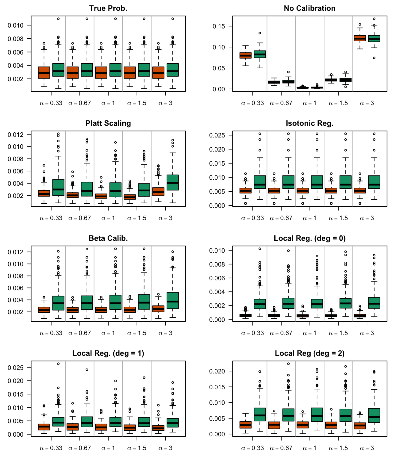
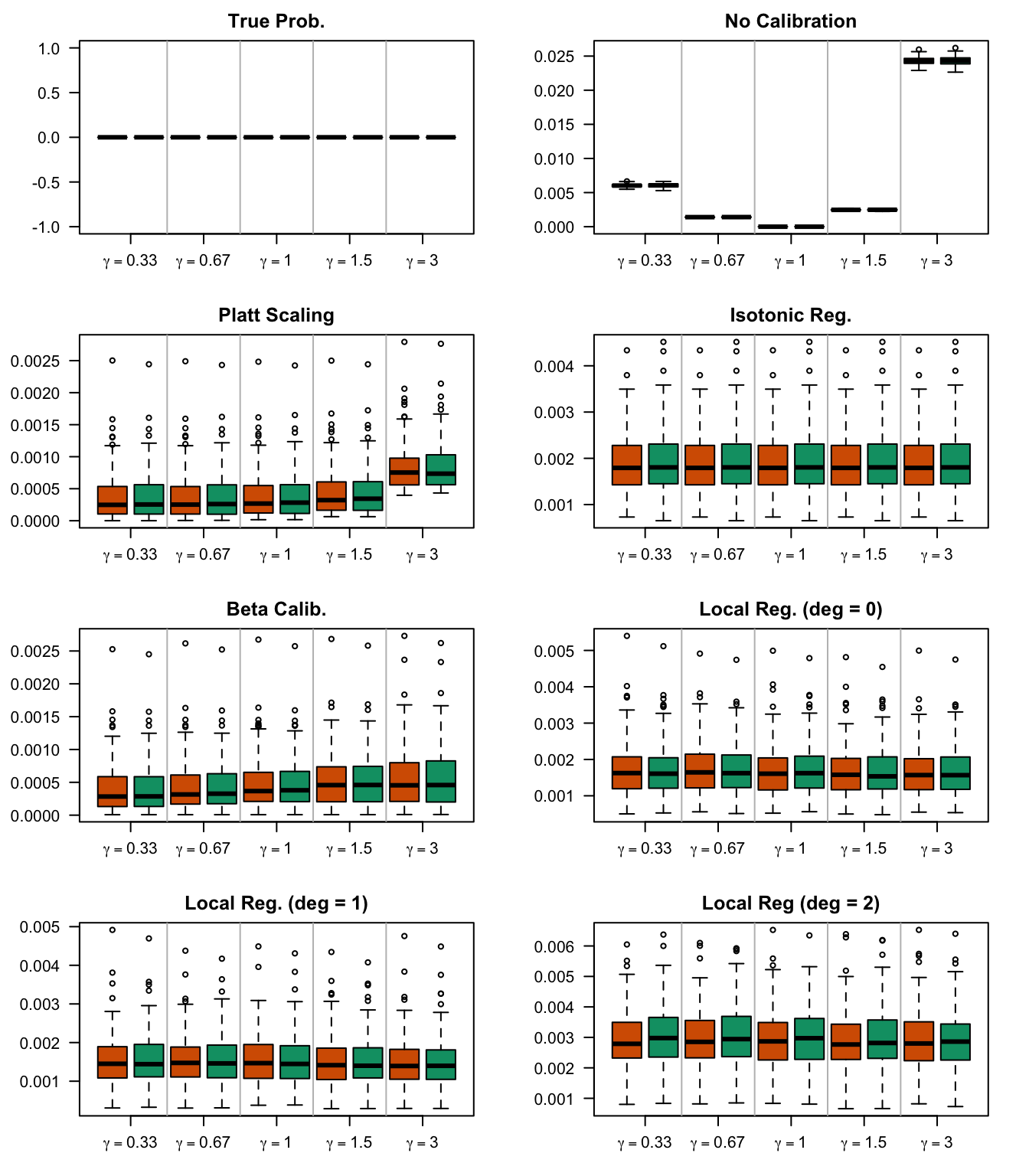
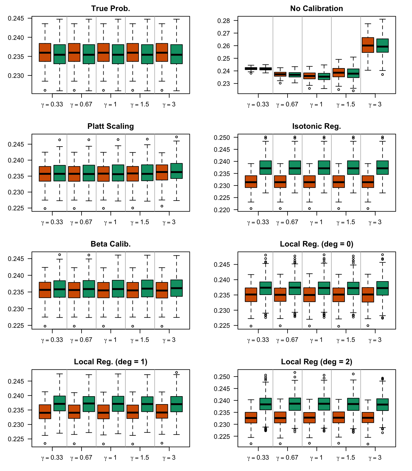
Let us define a function that computes the different calibration metrics for a single replication of the simulations.
#' Computes the calibration metrics for a set of observed and predicted #' probabilities#' #' @param obs observed events#' @param scores predicted scores#' @param true_probas true probabilities from the PGD (to compute MSE)#' @param linspace vector of values at which to compute the WMSEcompute_metrics <-function(obs, scores, true_probas, linspace) { mse <-mean((true_probas - scores)^2) brier <-brier_score(obs = obs, scores = scores)if (length(unique(scores)) >1) { ece <-e_calib_error(obs = obs, scores = scores, k =10, threshold = .5) qmse <-qmse_error(obs = obs, scores = scores, k =10, threshold = .5) } else { ece <-NA qmse <-NA } expected_events <-map(.x = linspace,.f =~local_ci_scores(obs = obs, scores = scores,tau = .x, nn = .15, prob = .95, method ="probit") ) |>bind_rows() wmse <-weighted_mse(local_scores = expected_events, scores = scores) lcs <-local_calib_score(obs = obs, scores = scores)tibble(mse = mse, brier = brier, ece = ece, qmse = qmse, wmse = wmse, lcs = lcs )}
Lastly, we define the f_simul() function to perform one simulation.
#' Performs one replication for a simulation#' #' @param i row number of the grid to use for the simulation#' @param grid grid tibble with the seed number (column `seed`) and the deformations value (either `alpha` or `gamma`)#' @param n_obs desired number of observation#' @param type deformation probability type (either `alpha` or `gamma`); the #' name should match with the `grid` tibble#' @param linspace values at which to compute the mean observed event when computing the WMSEf_simul <-function(i, grid, n_obs, type =c("alpha", "gamma"),linspace =NULL) {if (is.null(linspace)) linspace <-seq(0, 1, length.out =100)## 1. Generate Data---- current_seed <- grid$seed[i]if (type =="alpha") { transform_scale <- grid$alpha[i] current_data <-get_samples(seed = current_seed, n_obs = n_obs, alpha = transform_scale, gamma =1 ) } elseif (type =="gamma") { transform_scale <- grid$gamma[i] current_data <-get_samples(seed = current_seed, n_obs = n_obs, alpha =1, gamma = transform_scale ) } else {stop("Transform type should be either alpha or gamma.") }## 2. Calibration/Test sets----# Datasets with true probabilities data_all_calib <- current_data$data_all |>slice(current_data$calib_index) data_all_test <- current_data$data_all |>slice(-current_data$calib_index)## 3. Recalibration---- methods <-c("platt", "isotonic", "beta", "locfit", "locfit", "locfit") params <-list(NULL, NULL, NULL, list(nn = .15, deg =0), list(nn = .15, deg =1), list(nn = .15, deg =2) ) method_names <-c("platt", "isotonic", "beta", "locfit_0", "locfit_1", "locfit_2" ) res_recalibration <-map2(.x = methods,.y = params,.f =~recalibrate(obs_calib = data_all_calib$d, scores_calib = data_all_calib$p_u, obs_test = data_all_test$d, scores_test = data_all_test$p_u,method = .x,iso_params = .y,linspace = linspace ) )names(res_recalibration) <- method_names## 4. Calibration metrics----### Using True Probabilities#### Calibration Set calib_metrics_true_calib <-compute_metrics(obs = data_all_calib$d, scores = data_all_calib$p, true_probas = data_all_calib$p,linspace = linspace) |>mutate(method ="True Prob.", sample ="Calibration")#### Test Set calib_metrics_true_test <-compute_metrics(obs = data_all_test$d, scores = data_all_test$p, true_probas = data_all_test$p,linspace = linspace) |>mutate(method ="True Prob.", sample ="Test")### Without Recalibration#### Calibration Set calib_metrics_without_calib <-compute_metrics(obs = data_all_calib$d, scores = data_all_calib$p_u, true_probas = data_all_calib$p,linspace = linspace) |>mutate(method ="No Calibration", sample ="Calibration")#### Test Set calib_metrics_without_test <-compute_metrics(obs = data_all_test$d, scores = data_all_test$p_u, true_probas = data_all_test$p,linspace = linspace) |>mutate(method ="No Calibration", sample ="Test") calib_metrics <- calib_metrics_true_calib |>bind_rows(calib_metrics_true_test) |>bind_rows(calib_metrics_without_calib) |>bind_rows(calib_metrics_without_test)### With Recalibration: loop on methodsfor (method in method_names) { res_recalibration_current <- res_recalibration[[method]]#### Calibration Set calib_metrics_without_calib <-compute_metrics(obs = data_all_calib$d, scores = res_recalibration_current$tb_score_c_calib$p_c, true_probas = data_all_calib$p,linspace = linspace) |>mutate(method = method, sample ="Calibration")#### Test Set calib_metrics_without_test <-compute_metrics(obs = data_all_test$d, scores = res_recalibration_current$tb_score_c_test$p_c, true_probas = data_all_test$p,linspace = linspace) |>mutate(method = method, sample ="Test") calib_metrics <- calib_metrics |>bind_rows(calib_metrics_without_calib) |>bind_rows(calib_metrics_without_test) } calib_metrics <- calib_metrics |>mutate(seed = current_seed,transform_scale = transform_scale,type = type )list(res_recalibration = res_recalibration,linspace = linspace,calib_metrics = calib_metrics,data_all_calib = data_all_calib,data_all_test = data_all_test,seed = current_seed )}
2.4 Running the Simulations
Let us now run the simulations. We consider the following values for \(\alpha\) and \(\gamma\):
alphas <- gammas <-c(1/3, 2/3, 1, 3/2, 3)
For each value of \(\alpha\), and then for each value of \(\gamma\), let us make 200 replication samples from the same DGP.
n_repl <-200# number of replicationsn_obs <-2000# number of observations to drawgrid_alpha <-expand_grid(alpha = alphas, seed =1:n_repl)grid_gamma <-expand_grid(gamma = gammas, seed =1:n_repl)
We perform the simulations for the varying values of \(\alpha\)
We (re)define the function compute_gof_simul() to apply compute_gof(), defined above, to compute the different standard performance metrics on recalibrated probabilities (see Section 1.4 in Chapter 1), to which, initially, we have applied transformations:
#' Computes goodness of fit metrics for a replication#'#' @param i row number of the grid to use for the simulation#' @param grid grid tibble with the seed number (column `seed`) and the deformations value (either `alpha` or `gamma`)#' @param n_obs desired number of observation#' @param type deformation probability type (either `alpha` or `gamma`); the #' name should match with the `grid` tibblecompute_gof_simul <-function(i, grid, n_obs,type =c("alpha", "gamma")) { current_seed <- grid$seed[i]if (type =="alpha") { transform_scale <- grid$alpha[i] current_data <-get_samples(seed = current_seed, n_obs = n_obs, alpha = transform_scale, gamma =1 ) } elseif (type =="gamma") { transform_scale <- grid$gamma[i] current_data <-get_samples(seed = current_seed, n_obs = n_obs, alpha =1, gamma = transform_scale ) } else {stop("Transform type should be either alpha or gamma.") }# Get the calib/test datasets with true probabilities data_all_calib <- current_data$data_all |>slice(current_data$calib_index) data_all_test <- current_data$data_all |>slice(-current_data$calib_index)# Calibration set true_prob_calib <- data_all_calib$p_u obs_calib <- data_all_calib$d pred_calib <- data_all_calib$p# Test set true_prob_test <- data_all_test$p_u obs_test <- data_all_test$d pred_test <- data_all_test$p# Recalibration methods <-c("platt", "isotonic", "beta", "locfit", "locfit", "locfit") params <-list(NULL, NULL, NULL, list(nn = .15, deg =0), list(nn = .15, deg =1), list(nn = .15, deg =2) ) method_names <-c("platt", "isotonic", "beta", "locfit_0", "locfit_1", "locfit_2" ) res_recalibration <-map2(.x = methods,.y = params,.f =~recalibrate(obs_calib = data_all_calib$d, scores_calib = data_all_calib$p_u, obs_test = data_all_test$d, scores_test = data_all_test$p_u,method = .x,iso_params = .y,linspace =NULL ) )names(res_recalibration) <- method_names# Initialisation gof_metrics_simul_calib <-tibble() gof_metrics_simul_test <-tibble()# Calculate standard metrics## With Recalibration: loop on methodsfor (method in method_names) { res_recalibration_current <- res_recalibration[[method]]### Computation of metrics on the calibration set metrics_simul_calib <-map(.x =seq(0, 1, by = .01), # we vary the probability threshold.f =~compute_gof(true_prob = true_prob_calib,obs = obs_calib,#### the predictions are now recalibrated:pred = res_recalibration_current$tb_score_c_calib$p_c,threshold = .x ) ) |>list_rbind()### Computation of metricson the test set metrics_simul_test <-map(.x =seq(0, 1, by = .01), # we vary the probability threshold.f =~compute_gof(true_prob = true_prob_test,obs = obs_test,#### the predictions are now recalibrated:pred = res_recalibration_current$tb_score_c_test$p_c,threshold = .x ) ) |>list_rbind() roc_calib <- pROC::roc( obs_calib, res_recalibration_current$tb_score_c_calib$p_c ) auc_calib <-as.numeric(pROC::auc(roc_calib)) roc_test <- pROC::roc( obs_test, res_recalibration_current$tb_score_c_test$p_c ) auc_test <-as.numeric(pROC::auc(roc_test)) metrics_simul_calib <- metrics_simul_calib |>mutate(auc = auc_calib,seed = current_seed,scale_parameter = transform_scale,type = type,method = method,sample ="calibration" ) metrics_simul_test <- metrics_simul_test |>mutate(auc = auc_test,seed = current_seed,scale_parameter = transform_scale,type = type,method = method,sample ="test" ) gof_metrics_simul_calib <- gof_metrics_simul_calib |>bind_rows(metrics_simul_calib) gof_metrics_simul_test <- gof_metrics_simul_test |>bind_rows(metrics_simul_test) } gof_metrics_simul_calib |>bind_rows(gof_metrics_simul_test)}
Let us apply the function compute_gof_simul to the different simulations. We begin with the recalibrated probabilities initially transformed according to the variation of the parameter \(\alpha\).
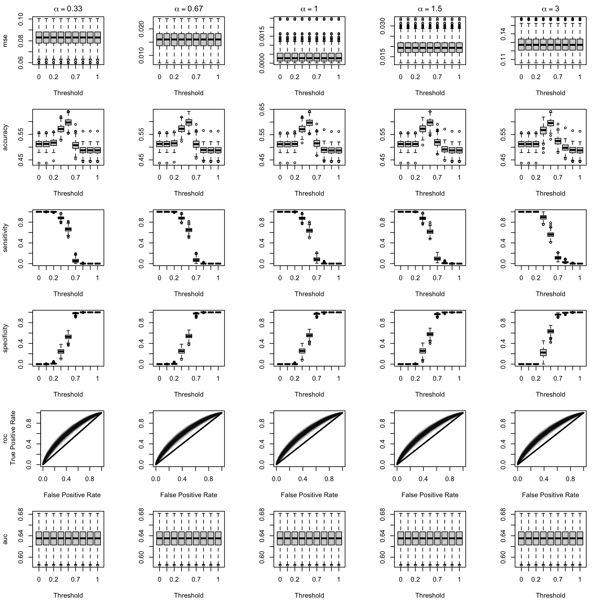
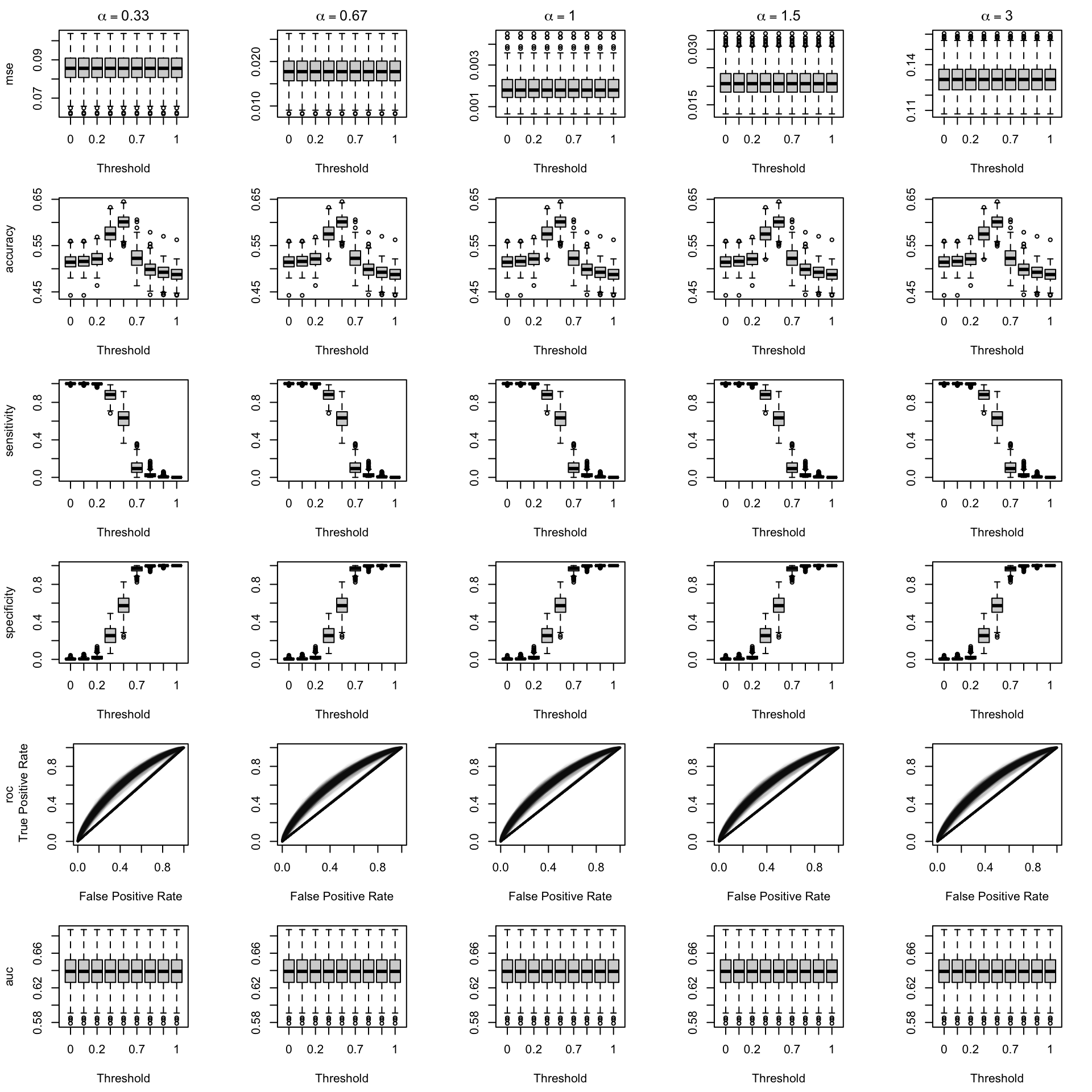
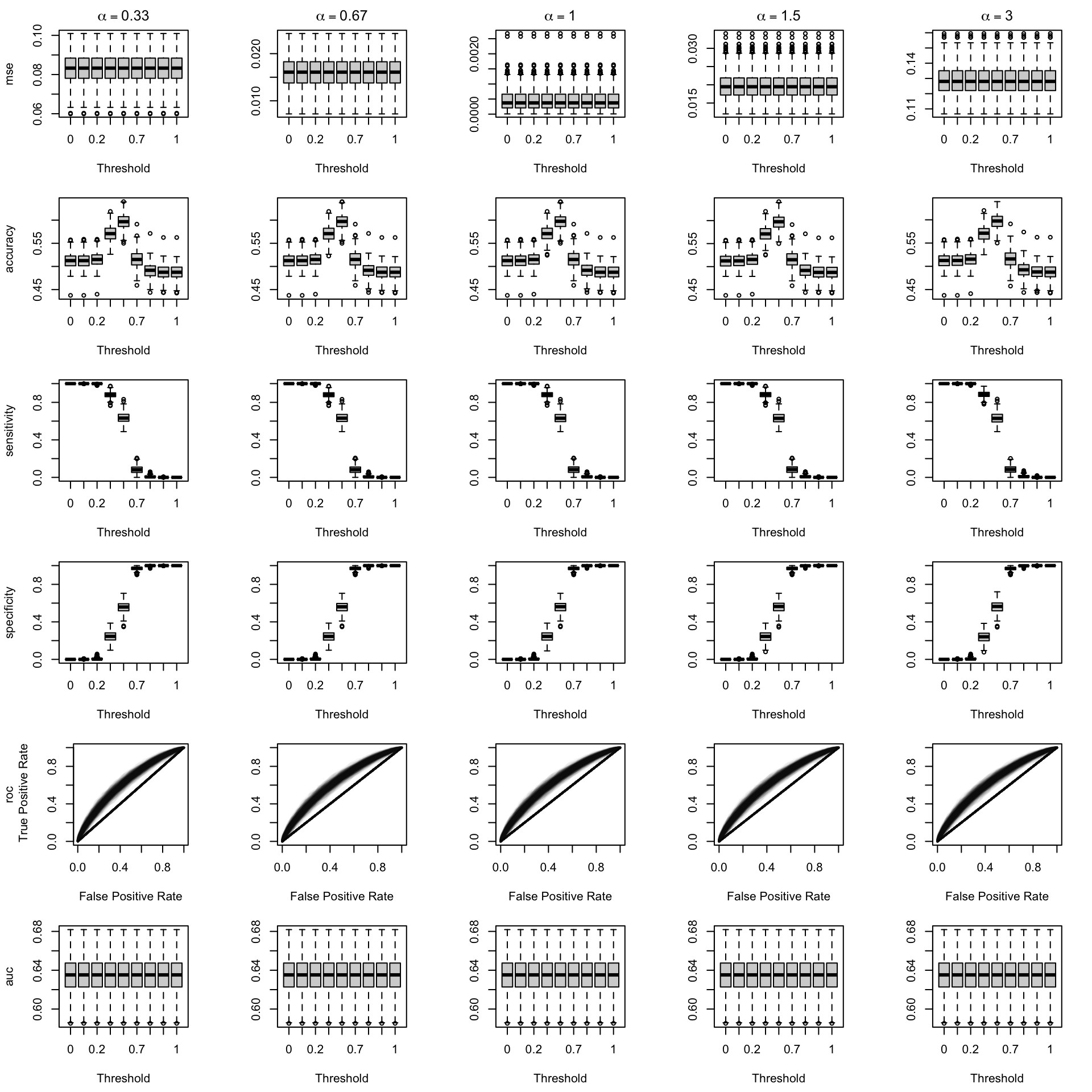
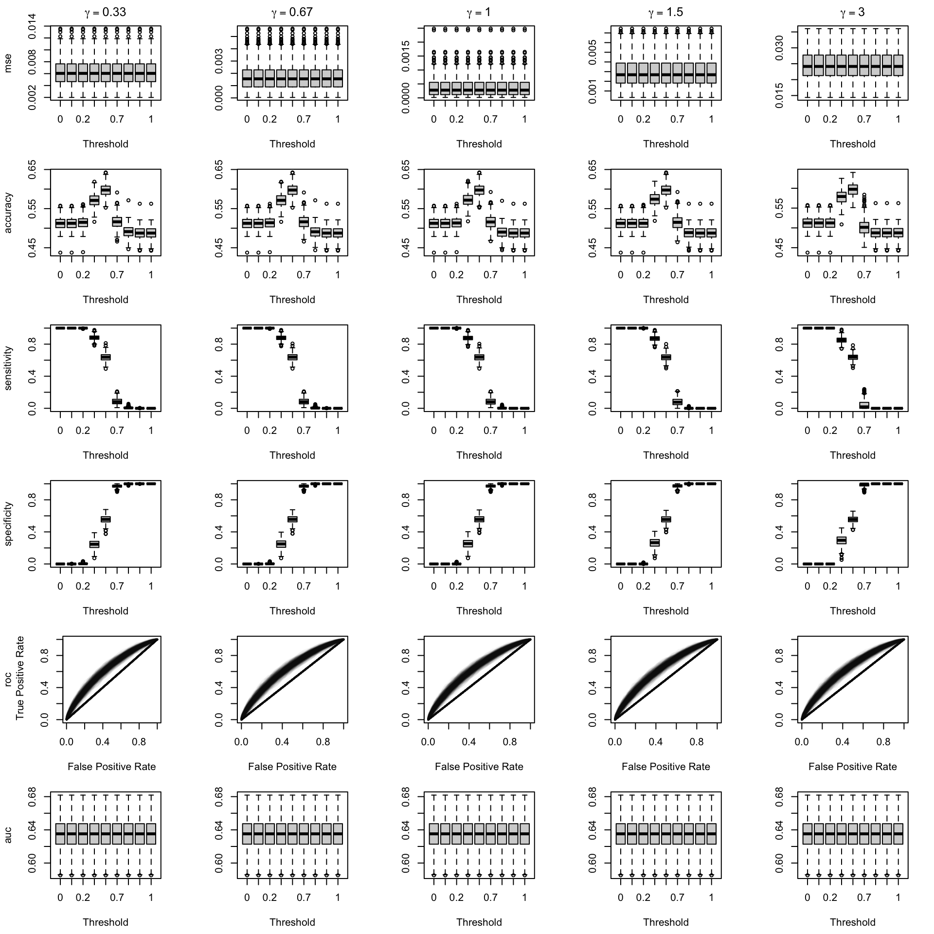
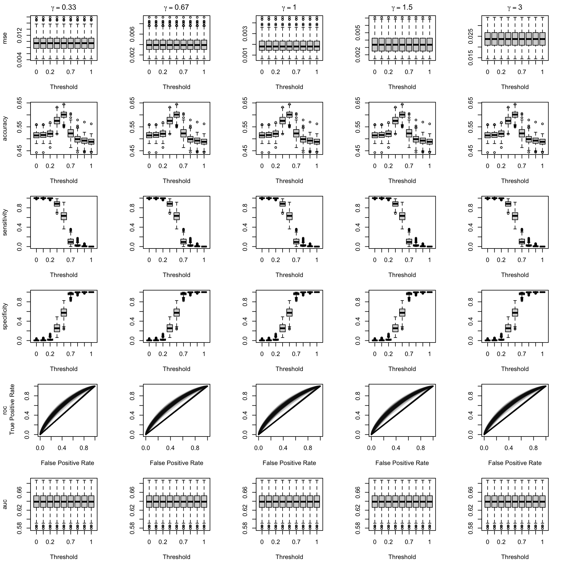
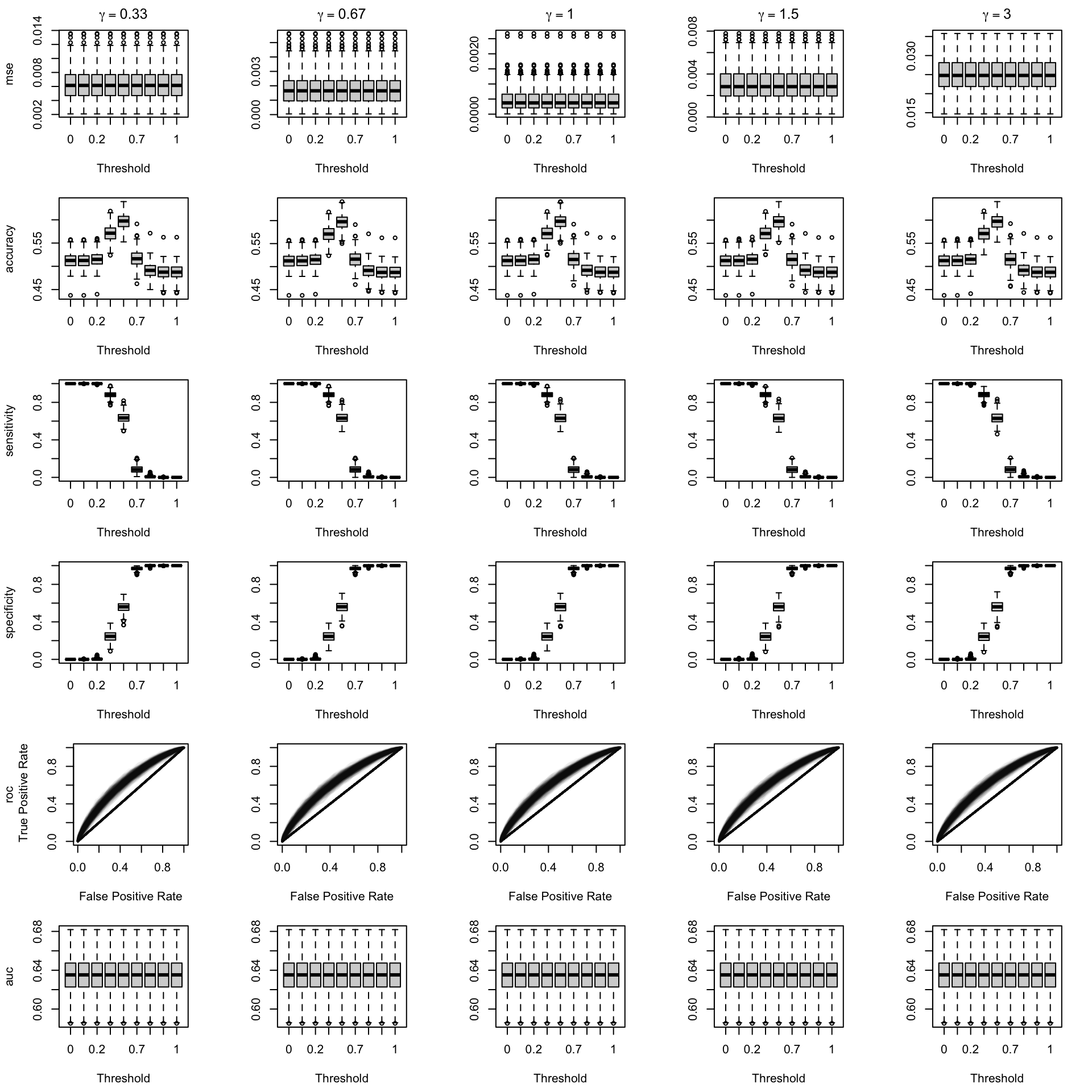
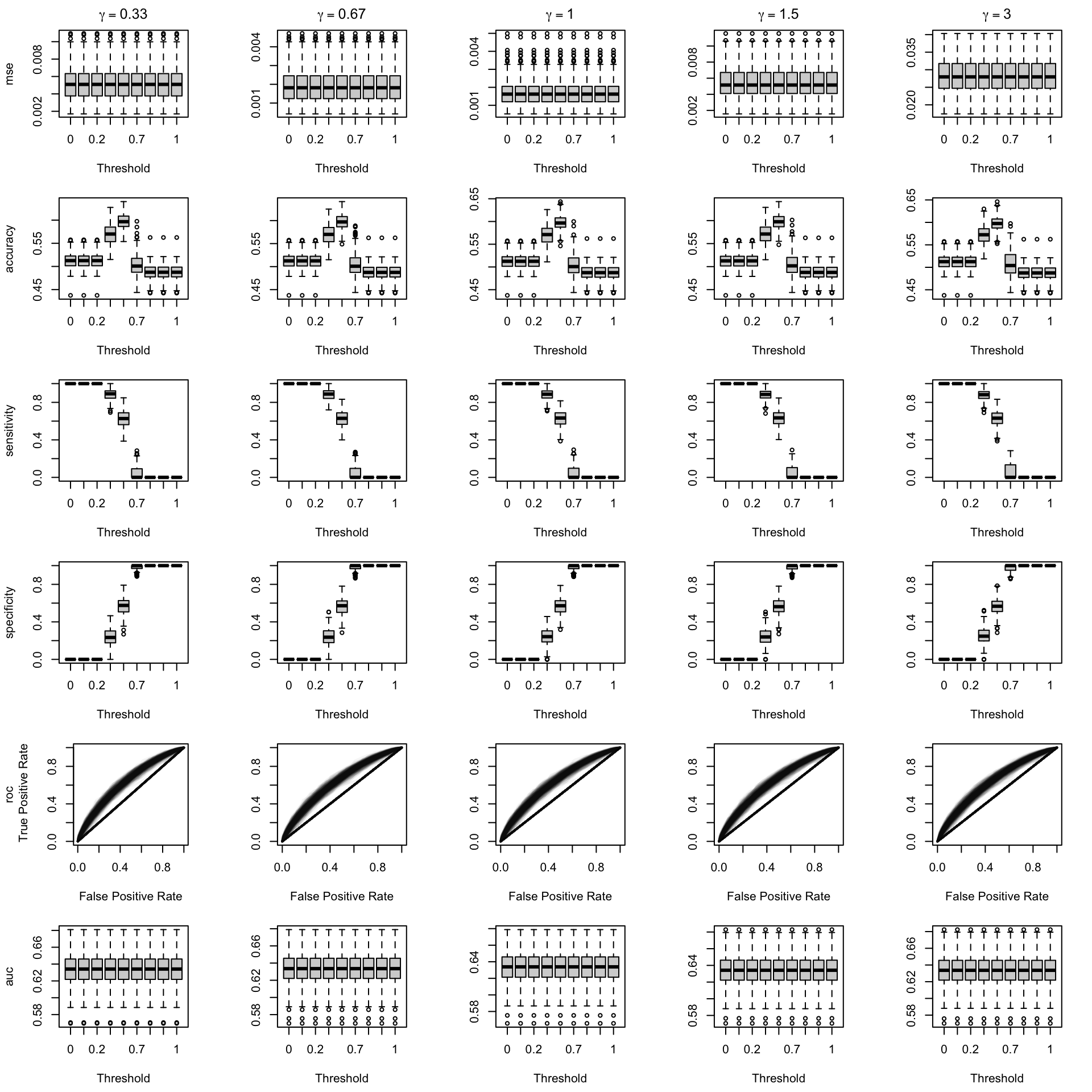
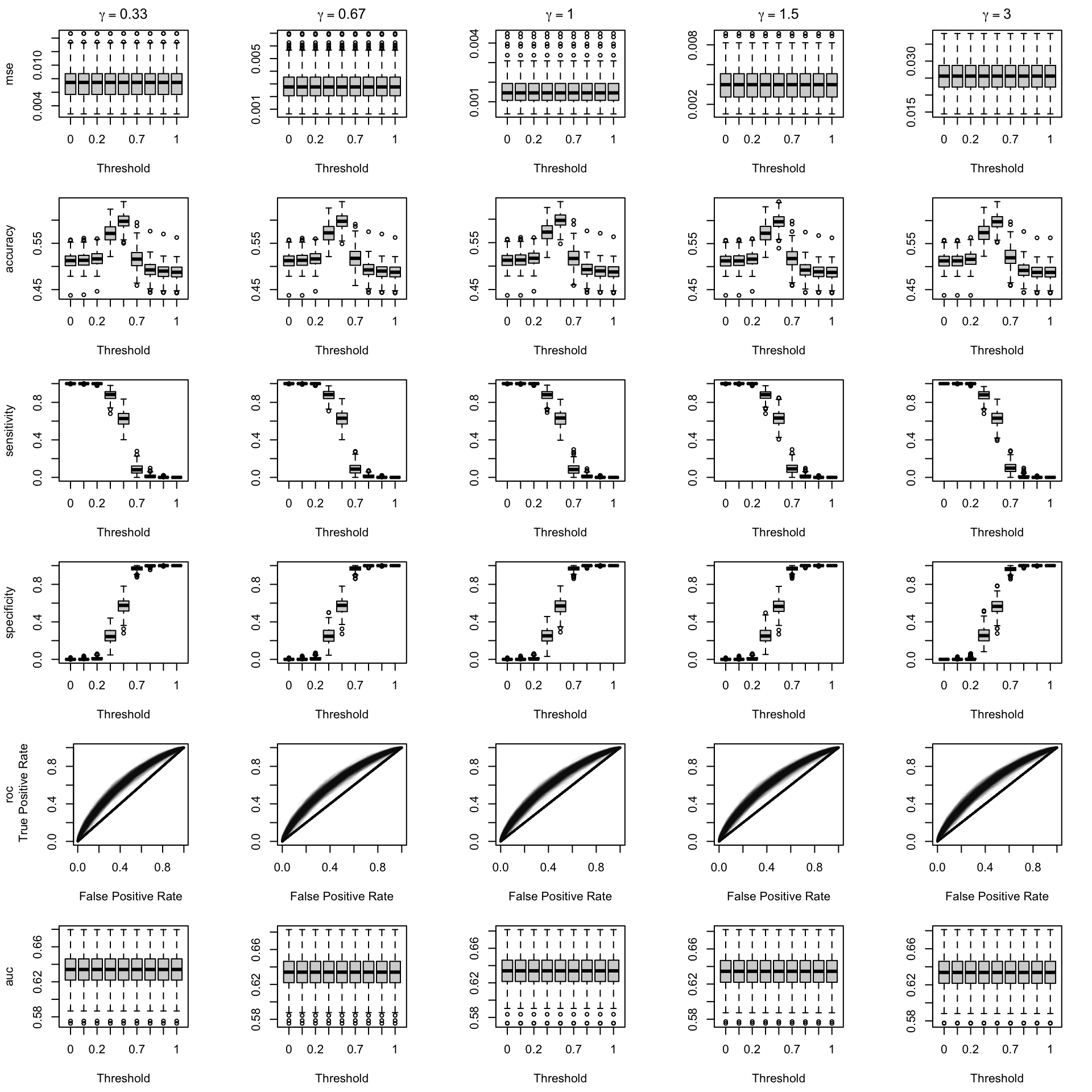
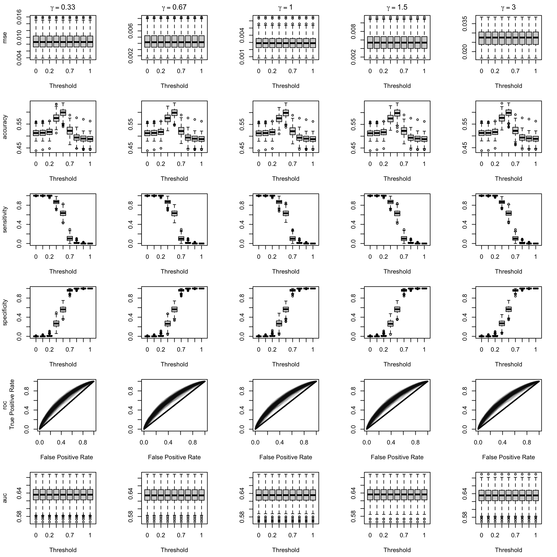
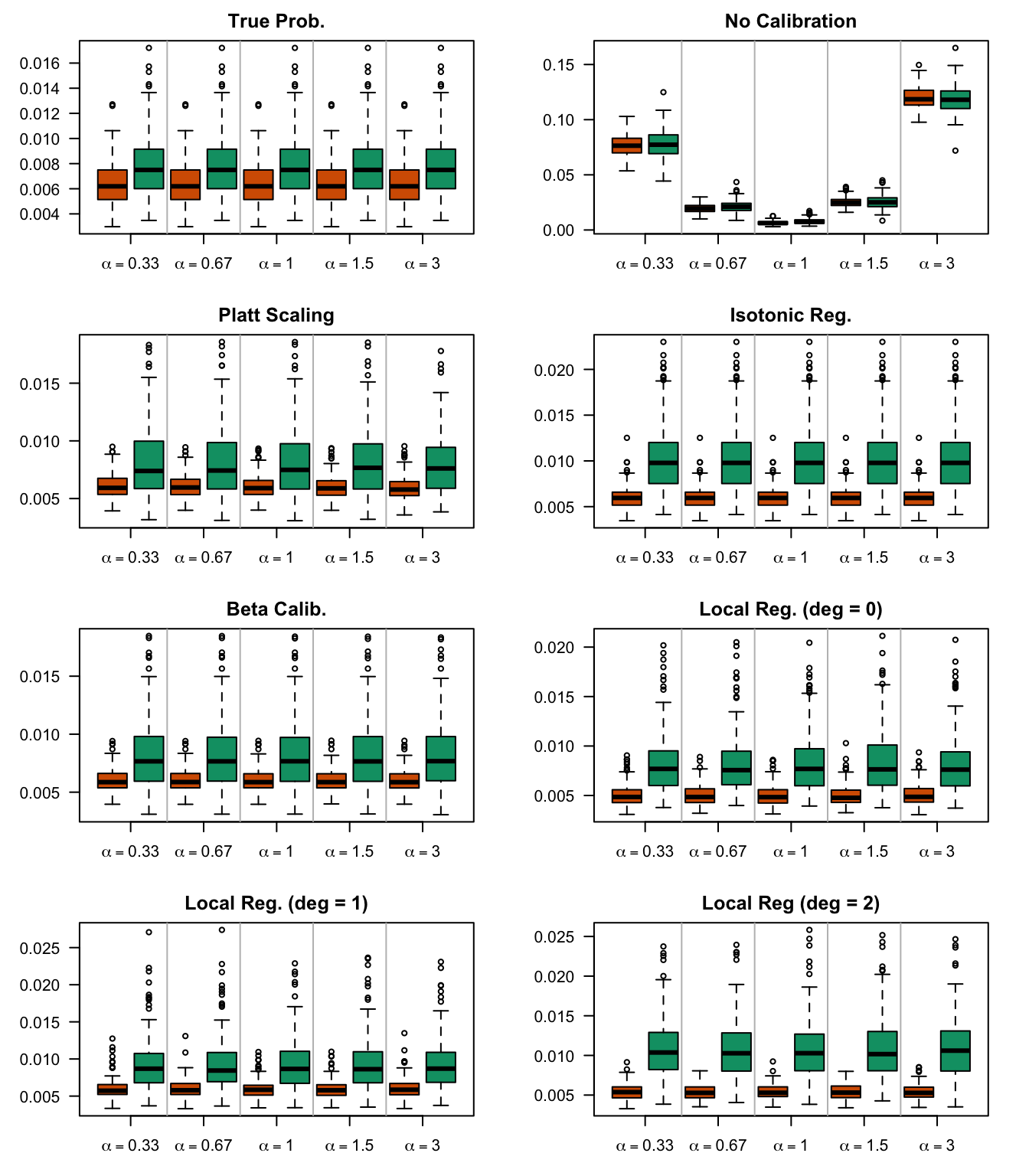
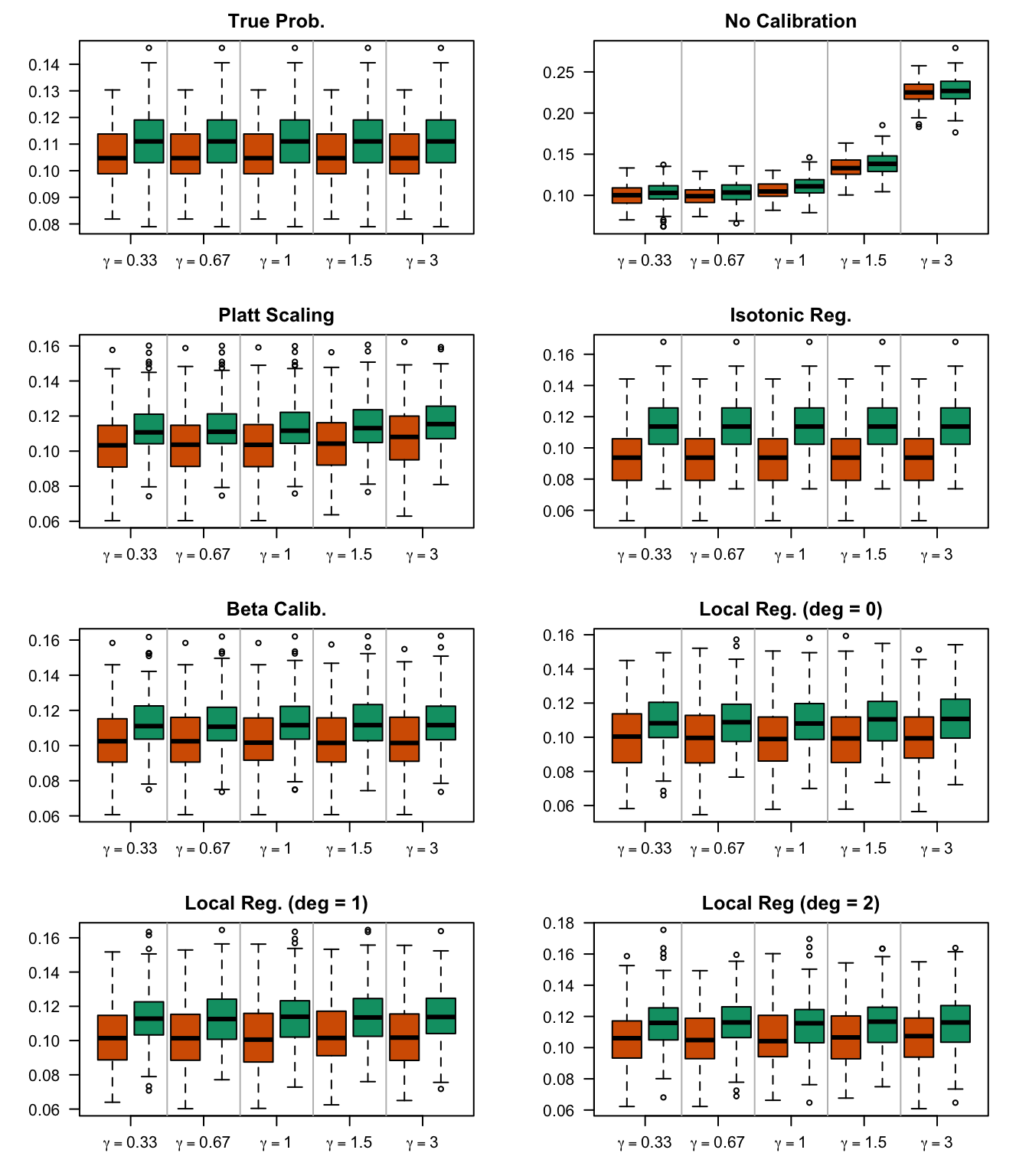
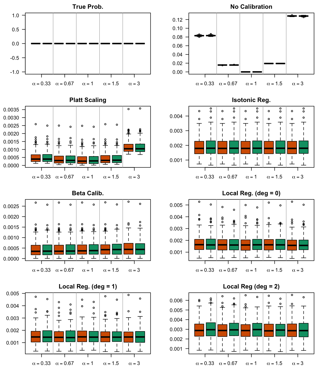
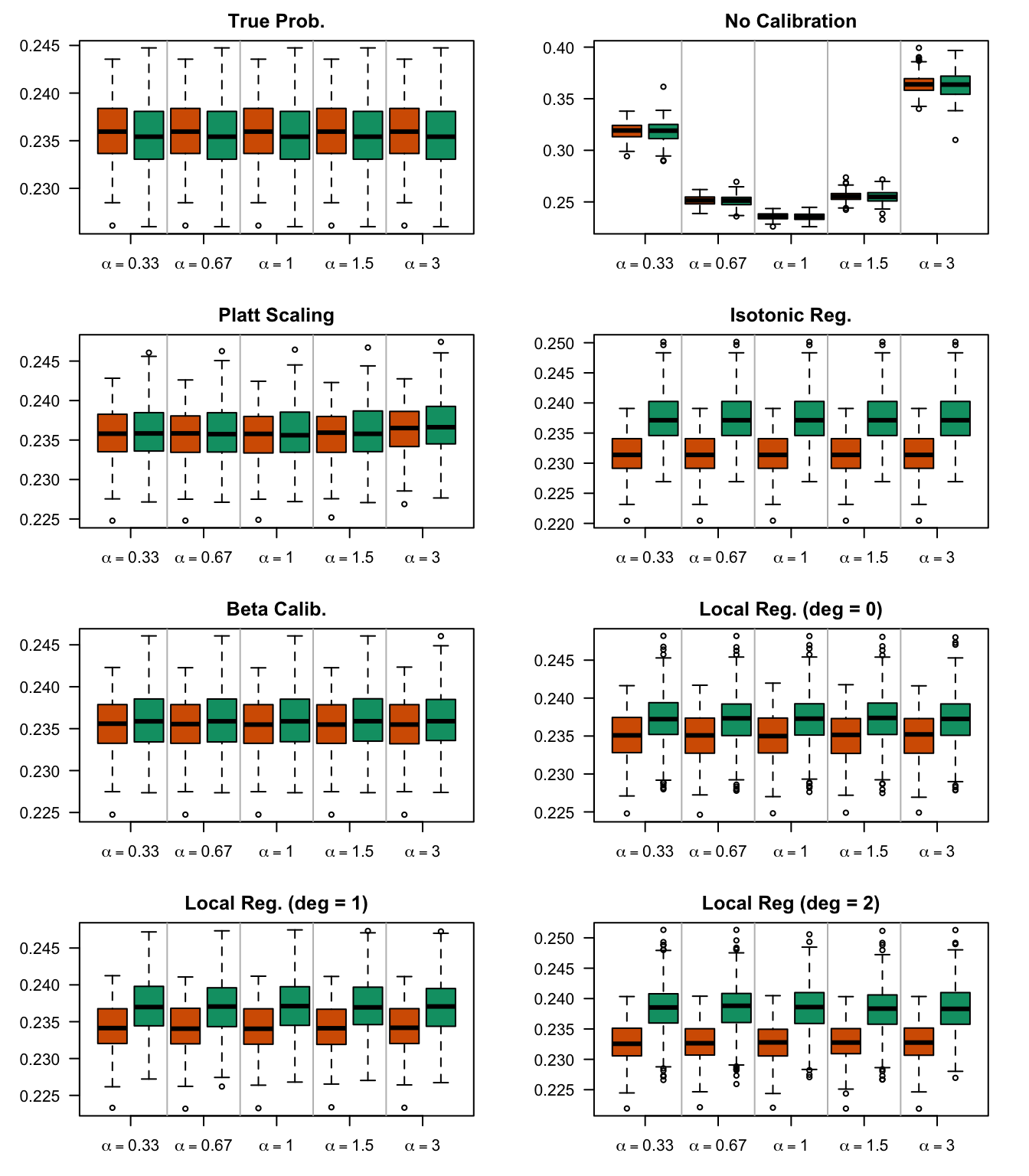
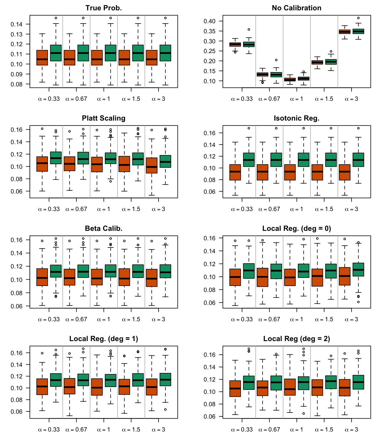
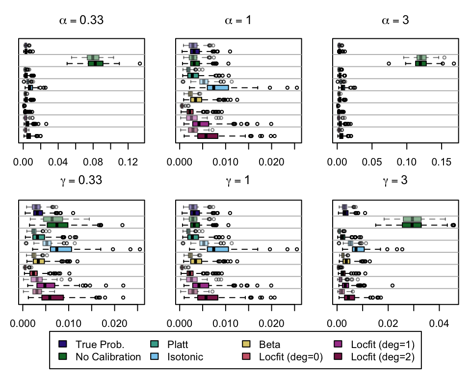
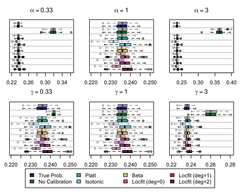
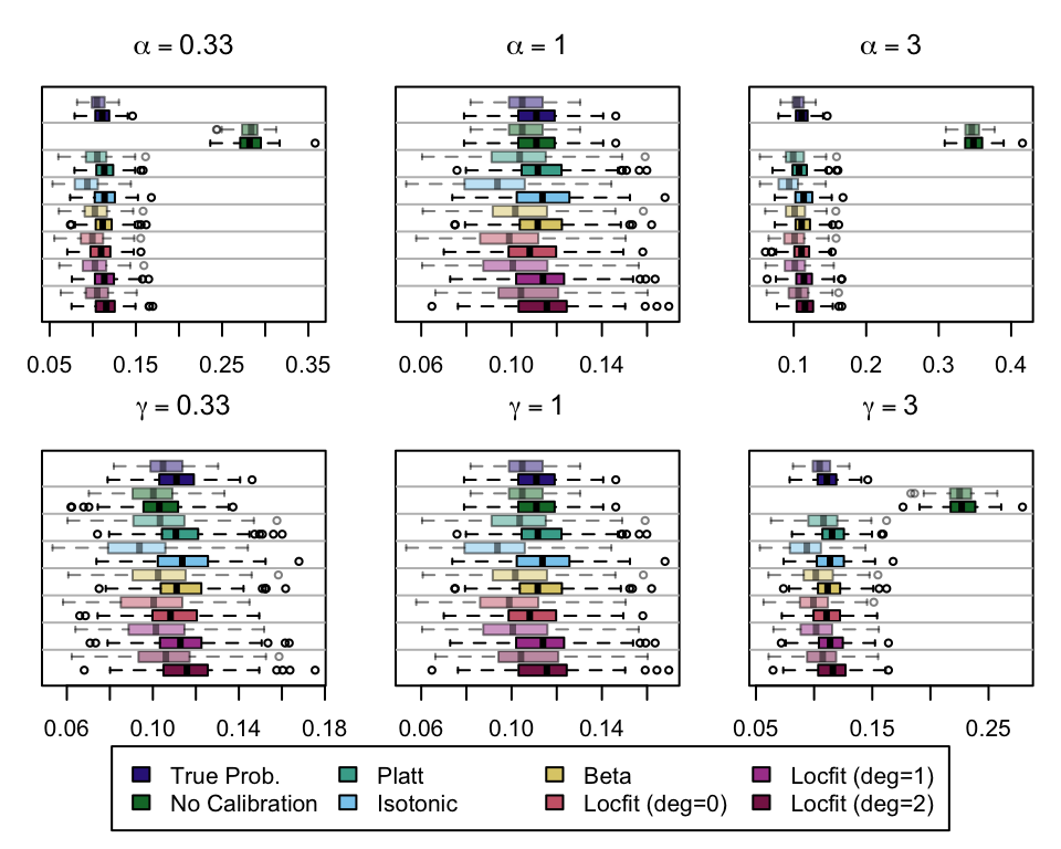
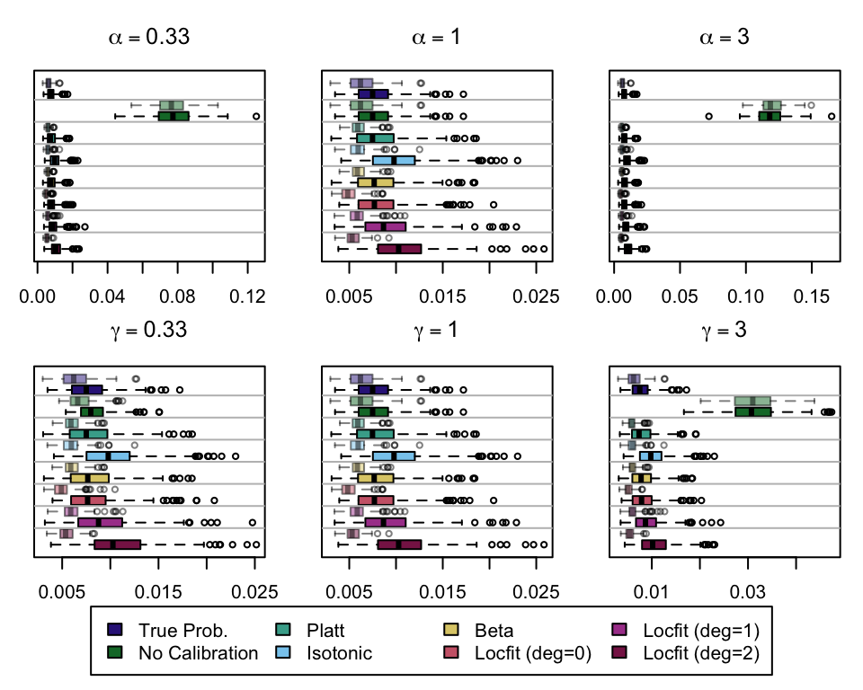
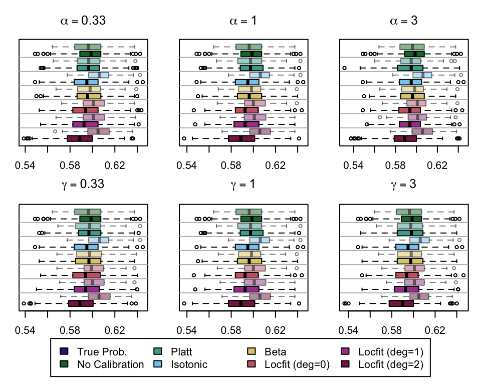
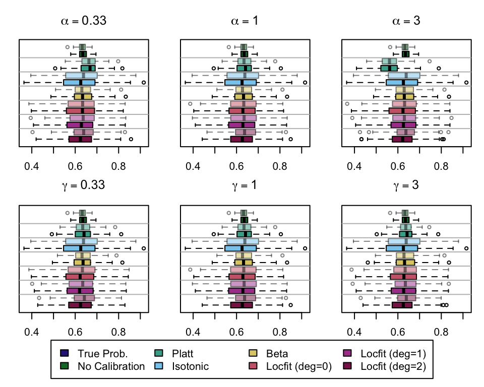
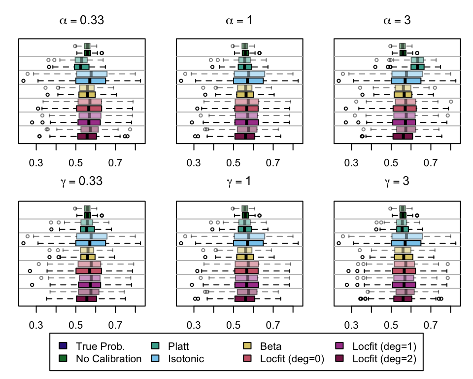
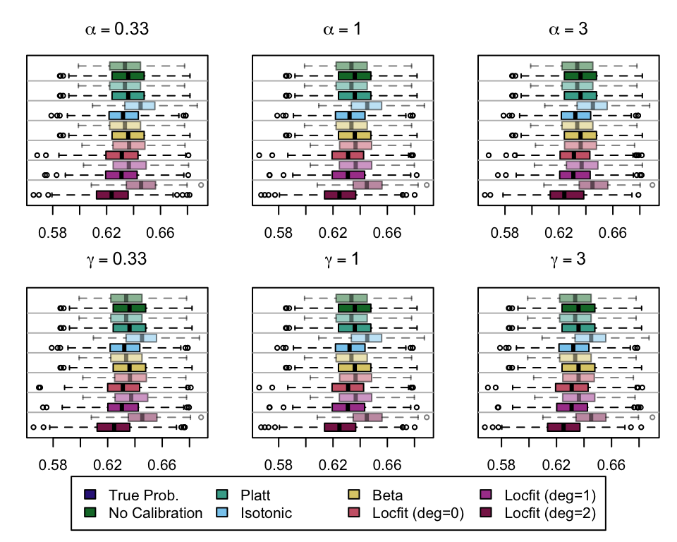
We (re)define function boxplot_simuls_metrics() from Section 1.4 (Chapter 1) to plot the standard metrics results on the recalibrated simulations. This function will produce a panel of boxplots. Each row of the panel will correspond to a metric whereas each column will correspond to a value for either \(\alpha\) or \(\gamma\). We also have one column for each recalibration method used. On each figure, the x-axis will correspond to the value used for the probability threshold \(\tau\), and the y-axis will correspond to the values of the metric.
#' Boxplots for the simulations to visualize the distribution of some #' traditional metrics as a function of the probability threshold.#' And, ROC curves#' The resulting figure is a panel of graphs, with vayring values for the #' transformation applied to the probabilities (in columns) and different #' metrics (in rows).#' #' @param tb_metrics tibble with computed metrics for the simulations#' @param type type of transformation: `"alpha"` or `"gamma"`#' @param metrics names of the metrics computedboxplot_simuls_metrics <-function(tb_metrics,type =c("alpha", "gamma"), metrics) { scale_parameters <-unique(tb_metrics$scale_parameter)par(mfrow =c(length(metrics), length(scale_parameters)))for (i_metric in1:length(metrics)) { metric <- metrics[i_metric]for (i_scale_parameter in1:length(scale_parameters)) { scale_parameter <- scale_parameters[i_scale_parameter] tb_metrics_current <- tb_metrics |>filter(scale_parameter ==!!scale_parameter)if (metric =="roc") { seeds <-unique(tb_metrics_current$seed)if (i_metric ==1) {# first row title <- latex2exp::TeX(str_c("$\\", type, " = ", round(scale_parameter, 2), "$") ) size_top <-2.1 } elseif (i_metric ==length(metrics)) {# Last row title <-"" size_top <-1.1 } else { title <-"" size_top <-1.1 }if (i_scale_parameter ==1) {# first column y_lab <-str_c(metric, "\n True Positive Rate") size_left <-5.1 } else { y_lab <-"" size_left <-4.1 }par(mar =c(4.5, size_left, size_top, 2.1))plot(0:1, 0:1,type ="l", col =NULL,xlim =0:1, ylim =0:1,xlab ="False Positive Rate", ylab = y_lab,main ="" )for (i_seed in1:length(seeds)) { tb_metrics_current_seed <- tb_metrics_current |>filter(seed == seeds[i_seed])lines(x = tb_metrics_current_seed$FPR, y = tb_metrics_current_seed$sensitivity,lwd =2, col =adjustcolor("black", alpha.f = .04) ) }segments(0, 0, 1, 1, col ="black", lty =2) } else {# not ROC tb_metrics_current <- tb_metrics_current |>filter(threshold %in%seq(0, 1, by = .1)) form <-str_c(metric, "~threshold")if (i_metric ==1) {# first row title <- latex2exp::TeX(str_c("$\\", type, " = ", round(scale_parameter, 2), "$") ) size_top <-2.1 } elseif (i_metric ==length(metrics)) {# Last row title <-"" size_top <-1.1 } else { title <-"" size_top <-1.1 }if (i_scale_parameter ==1) {# first column y_lab <- metric } else { y_lab <-"" }par(mar =c(4.5, 4.1, size_top, 2.1))boxplot(formula(form), data = tb_metrics_current,xlab ="Threshold", ylab = y_lab,main = title ) } } }}
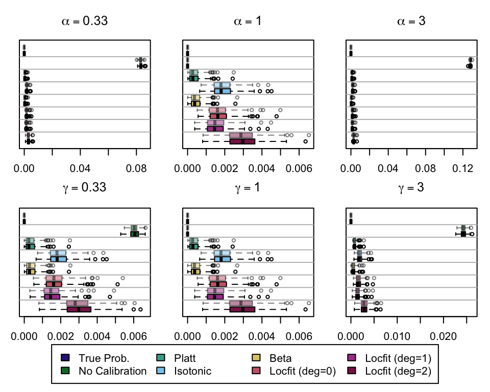
We aim to create a set of boxplots to visually assess the influence of probability transformations using \(\alpha\) or \(\gamma\) on standard metrics. Whenever \(\alpha \neq 1\) or \(\gamma \neq 1\), the resulting scores \(p^c\) represent values akin to those obtained from an initially uncalibrated model, with recalibration method applied. We want to verify that the recalibration methods applied to the uncalibrated probabilities do not degrade performance, as assessed by standard metrics. The results are shown in Figure 1.6 for vayring values of \(\alpha\), and in Figure 1.7 for vayring values of \(\gamma\).
Note
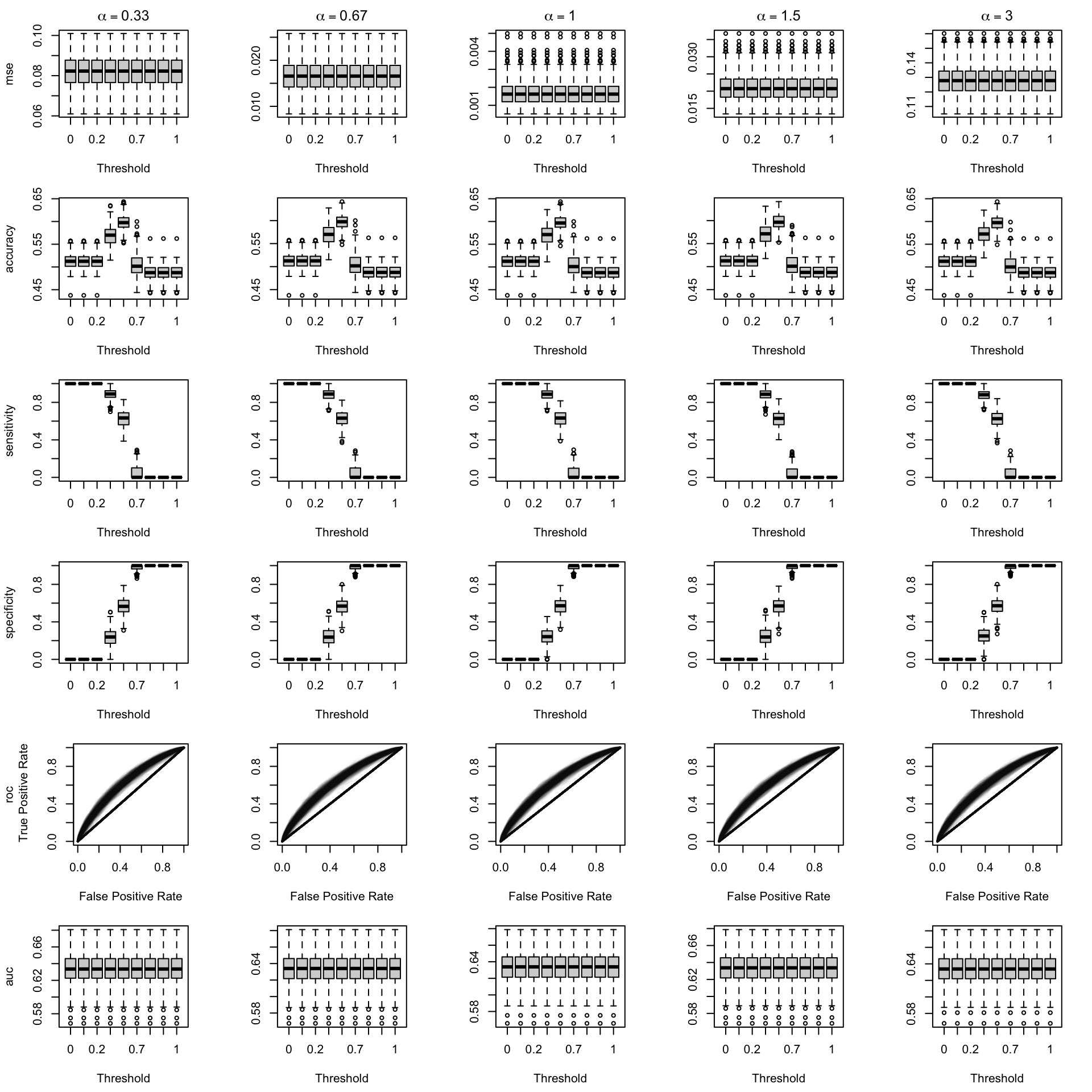
When using monotone transformation methods such as isotonic regression, the AUC cannot be degraded as it is insensitive to the application of an increasing function to the predicted scores by a model. Isotonic regression assumes that the initial model, without recalibration, has an AUC of 1. Therefore, if the initial model requires decreasing transformations in the recalibration step, isotonic regression will not be effective.
Figure 2.7: Calibration transformations made by varying \(\alpha\) and impact on standard metrics. The model is calibrated when \(\alpha=1\). The scores have been recalibrated using Platt-scaling.
Figure 2.8: Calibration transformations made by varying \(\alpha\) and impact on standard metrics. The model is calibrated when \(\alpha=1\). The scores have been recalibrated using Isotonic regression.
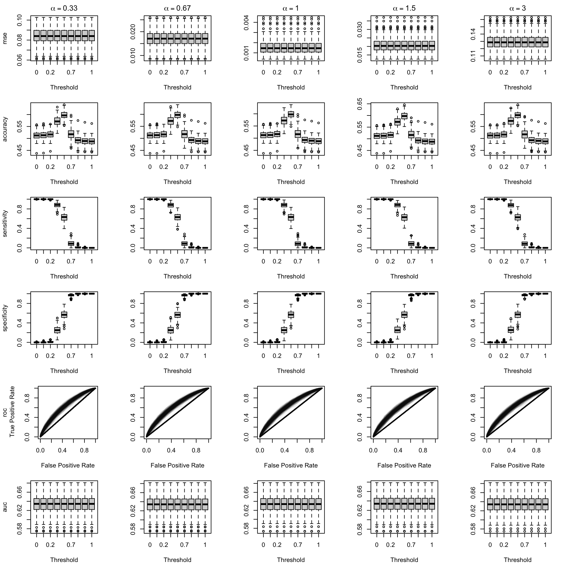
Figure 2.9: Calibration transformations made by varying \(\alpha\) and impact on standard metrics. The model is calibrated when \(\alpha=1\). The scores have been recalibrated using Beta calibration.
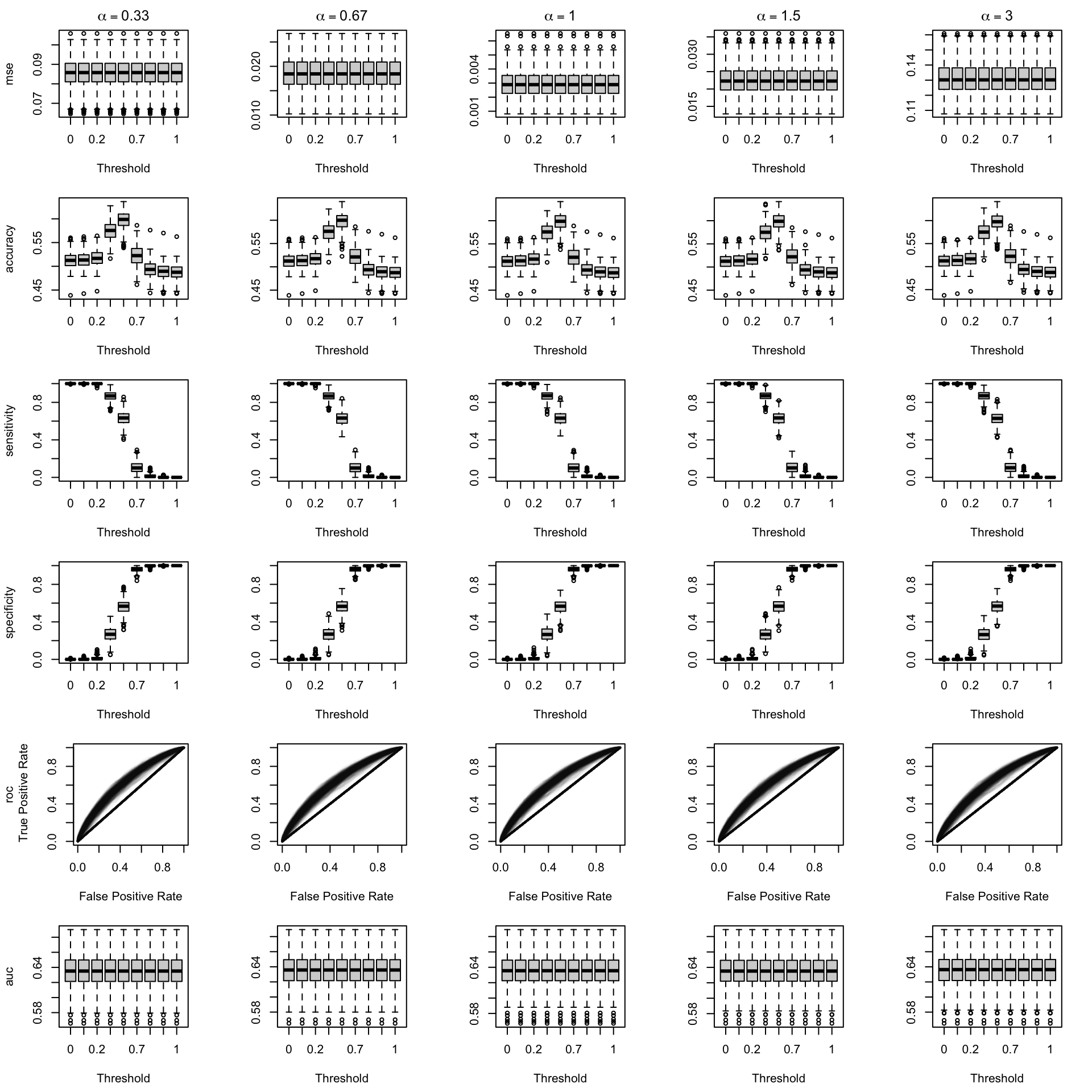
Figure 2.10: Calibration transformations made by varying \(\alpha\) and impact on standard metrics. The model is calibrated when \(\alpha=1\). The scores have been recalibrated using local regression (with deg=0).
Figure 2.11: Calibration transformations made by varying \(\alpha\) and impact on standard metrics. The model is calibrated when \(\alpha=1\). The scores have been recalibrated using local regression (with deg=1).
Figure 2.12: Calibration transformations made by varying \(\alpha\) and impact on standard metrics. The model is calibrated when \(\alpha=1\). The scores have been recalibrated using local regression (with deg=2).
Figure 2.13: Calibration transformations made by varying \(\gamma\) and impact on standard metrics. The model is calibrated when \(\beta=1\). The scores have been recalibrated using Platt-scaling.
Figure 2.14: Calibration transformations made by varying \(\gamma\) and impact on standard metrics. The model is calibrated when \(\beta=1\). The scores have been recalibrated using Isotonic regression.
Figure 2.15: Calibration transformations made by varying \(\gamma\) and impact on standard metrics. The model is calibrated when \(\beta=1\). The scores have been recalibrated using Beta calibration.
Figure 2.16: Calibration transformations made by varying \(\gamma\) and impact on standard metrics. The model is calibrated when \(\beta=1\). he scores have been recalibrated using local regression (with deg=0).
Figure 2.17: Calibration transformations made by varying \(\gamma\) and impact on standard metrics. The model is calibrated when \(\beta=1\). he scores have been recalibrated using local regression (with deg=1).
Figure 2.18: Calibration transformations made by varying \(\gamma\) and impact on standard metrics. The model is calibrated when \(\beta=1\). he scores have been recalibrated using local regression (with deg=0).
We can focus on the transformations that have degraded performance. For that purpose, we load the standard metrics computed on the uncalibrated probabilities:
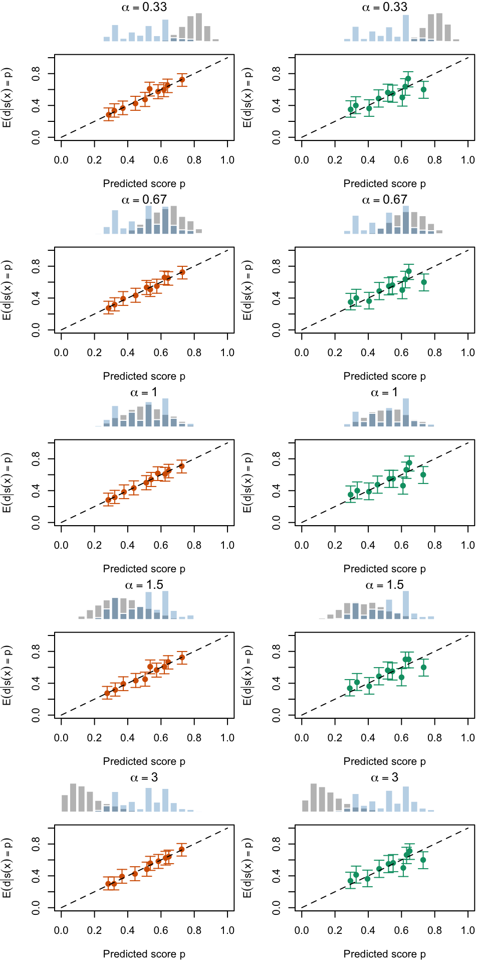
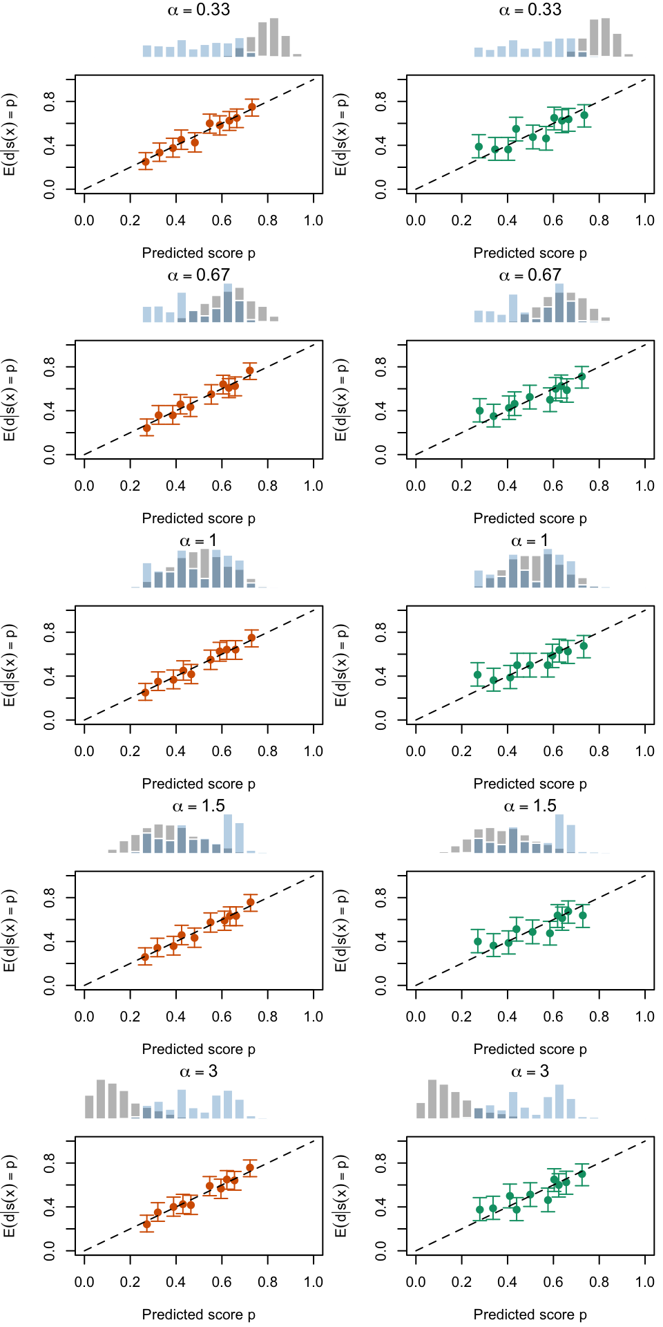
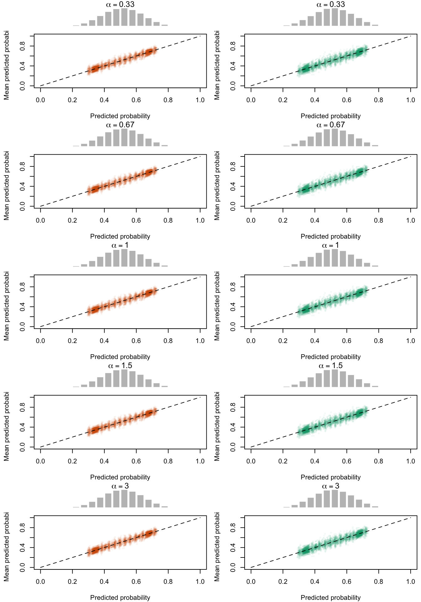
The x-axis of the calibration plot reports the mean predicted probabilities computed on different bins, where the bins are defined using the deciles of the predicted scores. On the y-axis, the corresponding fraction of positive events (\(d=1\)) are reported.
We can accompany the predictions made for each bin with a confidence interval, using the binom.confint() function from {binom}.
library(binom)
#' Confidence interval for binomial data, using quantile-defined bins#' #' @param obs vector of observed events#' @param scores vector of predicted probabilities#' @param k number of bins to create (quantiles, default to `10`)#' @param prob confidence interval level#' @param method Which method to use to construct the interval. Any combination #' of c("exact", "ac", "asymptotic", "wilson", "prop.test", "bayes", "logit", #' "cloglog", "probit") is allowed. Default is "all".#' @return a tibble with the following columns, where each row corresponds to#' a bin:#' - `mean`: estimation of $E(d | s(x) = p)$ where $p$ is the average score in bin b#' - `lower`: lower bound of the confidence interval#' - `upper`: upper bound of the confidence interval#' - `prediction`: average of `s(x)` in bin b#' - `score_class`: decile level of bin b#' - `nb`: number of observation in bin bci_scores_bins <-function(obs, scores, k,prob = .95, method ="probit" ) { summary_bins_calib <-get_summary_bins(obs = obs, scores = scores, k = k) new_k <-nrow(summary_bins_calib) prob_ic <-tibble(mean =rep(NA, new_k),lower =rep(NA, new_k),upper =rep(NA, new_k),prediction = summary_bins_calib |>pull("mean_score"),score_class = summary_bins_calib$score_class,nb = summary_bins_calib$nb )for (i in1:new_k) { prob_ic[i, 1:3] <-binom.confint(x = summary_bins_calib$sum_obs[i],n = summary_bins_calib$nb[i], conf.level = prob,methods = method )[, c("mean", "lower", "upper")] } prob_ic}
Let us define here a function to compute the confidence intervals for a single replication of our simulations.
We define a function, get_data_plot_quant_simul() to extract a desired simulation from our results (either from simul_recalib_alpha or from simul_recalib_gamma). The function get_data_plot_quant_simul() returns a list with two elements:
ci_res: the confidence interval for the calibration curve for the simulation
n_bins_scores: the counts of observation in each bin defined over [0,1] for the scores (uncalibrated or calibrated, for both the calibration set and the test set).
#' @param i index of the simulation to use (in `simul_recalib_alpha` or #' `simul_recalib_gamma`)#' @param type type of transformed probabilities (made on `alpha` or `gamma`)#' @param method name of the recalibration method to focus onget_data_plot_quant_simul <-function(i, type, method) {if (type =="alpha") { simul <- simul_recalib_alpha[[i]] transform_scale <- grid_alpha$alpha[i] } elseif (type =="gamma") { simul <- simul_recalib_gamma[[i]] transform_scale <- grid_gamma$gamma[i] } else {stop("Wrong value for argument `type`.") }# Counting number of obs in bins defined over [0,1] breaks <-seq(0, 1, by = .05)if (method =="True Prob.") { scores_calib <- simul$data_all_calib$p scores_test <- simul$data_all_test$p scores_c_calib <- scores_c_test <-NULL } elseif (method =="No Calibration") { scores_calib <- simul$data_all_calib$p_u scores_test <- simul$data_all_test$p_u scores_c_calib <- scores_c_test <-NULL } else { tb_score_c_calib <- simul$res_recalibration[[method]]$tb_score_c_calib tb_score_c_test <- simul$res_recalibration[[method]]$tb_score_c_test scores_calib <- tb_score_c_calib$p_u scores_test <- tb_score_c_test$p_u scores_c_calib <- tb_score_c_calib$p_c scores_c_test <- tb_score_c_test$p_c } n_bins_calib <-table(cut(scores_calib, breaks = breaks)) n_bins_test <-table(cut(scores_test, breaks = breaks))if (!is.null(scores_c_calib)) { n_bins_c_calib <-table(cut(scores_c_calib, breaks = breaks)) } else { n_bins_c_calib <-NA_integer_ }if (!is.null(scores_c_test)) { n_bins_c_test <-table(cut(scores_c_test, breaks = breaks)) } else { n_bins_c_test <-NA_integer_ } n_bins_scores <-tibble(bins =names(table(cut(breaks, breaks = breaks))),n_bins_calib =as.vector(n_bins_calib),n_bins_test =as.vector(n_bins_test),n_bins_c_calib =as.vector(n_bins_c_calib),n_bins_c_test =as.vector(n_bins_c_test),method = method,seed = simul$seed,type = type )# Confidence intervals ci_res <-conf_int_qbins_simul(simul = simul, method = method)list(ci_res = ci_res, n_bins_scores = n_bins_scores)}
Now, we can define a function that will plot the calibration maps computed on the calibration set and those computed on the test set. This function will plot a panel of calibration maps, each row corresponding to a specific value of the scale used to transform the probabilities (\(\alpha\) or \(\gamma\)). On top of each graph, we plot the histogram of uncalibrated scores and of calibrated scores.
In the Figures below, for the tabs True Pob. and No Calibration, the plots show the calibration curves obtained using the true probabilities and the uncalibrated scores instead of recalibrated scores. We do this for comparison purposes.
Calibration curves obtained using quantile-defined bins on the recalibrated scores for the calibration set (left) and for the test set (right) for varying values of \(\alpha\) for a single replication of the simulations. The histogram on top of each graph show the distribution of the uncalibrated scores, and that of the calibrated scores.
Calibration curves obtained using quantile-defined bins on the recalibrated scores for the calibration set (left) and for the test set (right) for varying values of \(\alpha\) for a single replication of the simulations. The histogram on top of each graph show the distribution of the uncalibrated scores, and that of the calibrated scores.
Calibration curves obtained using quantile-defined bins on the recalibrated scores for the calibration set (left) and for the test set (right) for varying values of \(\alpha\) for a single replication of the simulations. The histogram on top of each graph show the distribution of the uncalibrated scores, and that of the calibrated scores.
Calibration curves obtained using quantile-defined bins on the recalibrated scores for the calibration set (left) and for the test set (right) for varying values of \(\alpha\) for a single replication of the simulations. The histogram on top of each graph show the distribution of the uncalibrated scores, and that of the calibrated scores.
Calibration curves obtained using quantile-defined bins on the recalibrated scores for the calibration set (left) and for the test set (right) for varying values of \(\alpha\) for a single replication of the simulations. The histogram on top of each graph show the distribution of the uncalibrated scores, and that of the calibrated scores.
Calibration curves obtained using quantile-defined bins on the recalibrated scores for the calibration set (left) and for the test set (right) for varying values of \(\alpha\) for a single replication of the simulations. The histogram on top of each graph show the distribution of the uncalibrated scores, and that of the calibrated scores.
Calibration curves obtained using quantile-defined bins on the recalibrated scores for the calibration set (left) and for the test set (right) for varying values of \(\alpha\) for a single replication of the simulations. The histogram on top of each graph show the distribution of the uncalibrated scores, and that of the calibrated scores.
Calibration curves obtained using quantile-defined bins on the recalibrated scores for the calibration set (left) and for the test set (right) for varying values of \(\alpha\) for a single replication of the simulations. The histogram on top of each graph show the distribution of the uncalibrated scores, and that of the calibrated scores.
Calibration curves obtained using quantile-defined bins on the recalibrated scores for the calibration set (left) and for the test set (right) for varying values of \(\gamma\) for a single replication of the simulations. The histogram on top of each graph show the distribution of the uncalibrated scores, and that of the calibrated scores.
Calibration curves obtained using quantile-defined bins on the recalibrated scores for the calibration set (left) and for the test set (right) for varying values of \(\gamma\) for a single replication of the simulations. The histogram on top of each graph show the distribution of the uncalibrated scores, and that of the calibrated scores.
Calibration curves obtained using quantile-defined bins on the recalibrated scores for the calibration set (left) and for the test set (right) for varying values of \(\gamma\) for a single replication of the simulations. The histogram on top of each graph show the distribution of the uncalibrated scores, and that of the calibrated scores.
Calibration curves obtained using quantile-defined bins on the recalibrated scores for the calibration set (left) and for the test set (right) for varying values of \(\gamma\) for a single replication of the simulations. The histogram on top of each graph show the distribution of the uncalibrated scores, and that of the calibrated scores.
Calibration curves obtained using quantile-defined bins on the recalibrated scores for the calibration set (left) and for the test set (right) for varying values of \(\gamma\) for a single replication of the simulations. The histogram on top of each graph show the distribution of the uncalibrated scores, and that of the calibrated scores.
Calibration curves obtained using quantile-defined bins on the recalibrated scores for the calibration set (left) and for the test set (right) for varying values of \(\gamma\) for a single replication of the simulations. The histogram on top of each graph show the distribution of the uncalibrated scores, and that of the calibrated scores.
Calibration curves obtained using quantile-defined bins on the recalibrated scores for the calibration set (left) and for the test set (right) for varying values of \(\gamma\) for a single replication of the simulations. The histogram on top of each graph show the distribution of the uncalibrated scores, and that of the calibrated scores.
Calibration curves obtained using quantile-defined bins on the recalibrated scores for the calibration set (left) and for the test set (right) for varying values of \(\gamma\) for a single replication of the simulations. The histogram on top of each graph show the distribution of the uncalibrated scores, and that of the calibrated scores.
2.6.2 Calibration Curve with Moving Average
The calibration curves will computed using the local_ci_scores() (defined in Section 2.3.1) and accompanied by a confidence interval obtained using the binom.confint() function from {binom}.
Let us first focus on a single replication for which we can plot the calibration curve with its confidence interval.
For convenience, we create a function, get_data_plot_calib_ma_simul() that returns two elements::
tb_ci: confidence intervals associated with the calibration curve for a single replication
n_bins_scores: the count of observation in each bins defined over the [0,1] segment for the scores (uncalibrated and calibrated, for both the train set and the test set).
#' @param i index of the simulation to use (in `simul_recalib_alpha` or #' `simul_recalib_gamma`)#' @param type type of transformed probabilities (made on `alpha` or `gamma`)#' @param method name of the recalibration method to focus onget_data_plot_calib_ma_simul <-function(i, type, method) {if (type =="alpha") { simul <- simul_recalib_alpha[[i]] transform_scale <- grid_alpha$alpha[i] } elseif (type =="gamma") { simul <- simul_recalib_gamma[[i]] transform_scale <- grid_gamma$gamma[i] } else {stop("Wrong value for argument `type`.") }# Counting number of obs in bins defined over [0,1] breaks <-seq(0, 1, by = .05)if (method =="True Prob.") { scores_calib <- simul$data_all_calib$p scores_test <- simul$data_all_test$p scores_c_calib <- scores_c_test <-NULL } elseif (method =="No Calibration") { scores_calib <- simul$data_all_calib$p_u scores_test <- simul$data_all_test$p_u scores_c_calib <- scores_c_test <-NULL } else { tb_score_c_calib <- simul$res_recalibration[[method]]$tb_score_c_calib tb_score_c_test <- simul$res_recalibration[[method]]$tb_score_c_test scores_calib <- tb_score_c_calib$p_u scores_test <- tb_score_c_test$p_u scores_c_calib <- tb_score_c_calib$p_c scores_c_test <- tb_score_c_test$p_c } n_bins_calib <-table(cut(scores_calib, breaks = breaks)) n_bins_test <-table(cut(scores_test, breaks = breaks))if (!is.null(scores_c_calib)) { n_bins_c_calib <-table(cut(scores_c_calib, breaks = breaks)) } else { n_bins_c_calib <-NA_integer_ }if (!is.null(scores_c_test)) { n_bins_c_test <-table(cut(scores_c_test, breaks = breaks)) } else { n_bins_c_test <-NA_integer_ } n_bins_scores <-tibble(bins =names(table(cut(breaks, breaks = breaks))),n_bins_calib =as.vector(n_bins_calib),n_bins_test =as.vector(n_bins_test),n_bins_c_calib =as.vector(n_bins_c_calib),n_bins_c_test =as.vector(n_bins_c_test),method = method,seed = simul$seed,type = type )# Confidence intervals tb_ci <-calibration_curve_ma_simul(simul = simul, method = method, nn = .15, prob = .95, ci_method ="probit" )list(tb_ci = tb_ci,n_bins_scores = n_bins_scores )}
We define a function that will plot the calibration maps computed on the calibration set and those computed on the test set. This function will plot a panel of calibration maps, each row corresponding to a specific value of the scale used to transform the probabilities (\(\alpha\) or \(\gamma\)).
For the first two tabs, True Prob. and No Calibration, the calibration curves are those computed using the true probabilities and the uncalibrated scores instead of some recalibrated scores. This is done for comparison purposes.
Calibration curves obtained with recalibrated scores. The curves are obtained with a moving average for the calibration set (left) and for the test set (right) for varying values of \(\alpha\) for a single replication of the simulations. The histogram on top of each graph show the distribution of the uncalibrated scores, and that of the calibrated scores.
Calibration curves obtained with recalibrated scores. The curves are obtained with a moving average for the calibration set (left) and for the test set (right) for varying values of \(\alpha\) for a single replication of the simulations. The histogram on top of each graph show the distribution of the uncalibrated scores, and that of the calibrated scores.
Calibration curves obtained with recalibrated scores. The curves are obtained with a moving average for the calibration set (left) and for the test set (right) for varying values of \(\alpha\) for a single replication of the simulations. The histogram on top of each graph show the distribution of the uncalibrated scores, and that of the calibrated scores.
Calibration curves obtained with recalibrated scores. The curves are obtained with a moving average for the calibration set (left) and for the test set (right) for varying values of \(\alpha\) for a single replication of the simulations. The histogram on top of each graph show the distribution of the uncalibrated scores, and that of the calibrated scores.
Calibration curves obtained with recalibrated scores. The curves are obtained with a moving average for the calibration set (left) and for the test set (right) for varying values of \(\alpha\) for a single replication of the simulations. The histogram on top of each graph show the distribution of the uncalibrated scores, and that of the calibrated scores.
Calibration curves obtained with recalibrated scores. The curves are obtained with a moving average for the calibration set (left) and for the test set (right) for varying values of \(\alpha\) for a single replication of the simulations. The histogram on top of each graph show the distribution of the uncalibrated scores, and that of the calibrated scores.
Calibration curves obtained with recalibrated scores. The curves are obtained with a moving average for the calibration set (left) and for the test set (right) for varying values of \(\alpha\) for a single replication of the simulations. The histogram on top of each graph show the distribution of the uncalibrated scores, and that of the calibrated scores.
Calibration curves obtained with recalibrated scores. The curves are obtained with a moving average for the calibration set (left) and for the test set (right) for varying values of \(\alpha\) for a single replication of the simulations. The histogram on top of each graph show the distribution of the uncalibrated scores, and that of the calibrated scores.
Calibration curves obtained with recalibrated scores. The curves are obtained with a moving average for the calibration set (left) and for the test set (right) for varying values of \(\gamma\) for a single replication of the simulations. The histogram on top of each graph show the distribution of the uncalibrated scores, and that of the calibrated scores.
Calibration curves obtained with recalibrated scores. The curves are obtained with a moving average for the calibration set (left) and for the test set (right) for varying values of \(\gamma\) for a single replication of the simulations. The histogram on top of each graph show the distribution of the uncalibrated scores, and that of the calibrated scores.
Calibration curves obtained with recalibrated scores. The curves are obtained with a moving average for the calibration set (left) and for the test set (right) for varying values of \(\gamma\) for a single replication of the simulations. The histogram on top of each graph show the distribution of the uncalibrated scores, and that of the calibrated scores.
Calibration curves obtained with recalibrated scores. The curves are obtained with a moving average for the calibration set (left) and for the test set (right) for varying values of \(\gamma\) for a single replication of the simulations. The histogram on top of each graph show the distribution of the uncalibrated scores, and that of the calibrated scores.
Calibration curves obtained with recalibrated scores. The curves are obtained with a moving average for the calibration set (left) and for the test set (right) for varying values of \(\gamma\) for a single replication of the simulations. The histogram on top of each graph show the distribution of the uncalibrated scores, and that of the calibrated scores.
Calibration curves obtained with recalibrated scores. The curves are obtained with a moving average for the calibration set (left) and for the test set (right) for varying values of \(\gamma\) for a single replication of the simulations. The histogram on top of each graph show the distribution of the uncalibrated scores, and that of the calibrated scores.
Calibration curves obtained with recalibrated scores. The curves are obtained with a moving average for the calibration set (left) and for the test set (right) for varying values of \(\gamma\) for a single replication of the simulations. The histogram on top of each graph show the distribution of the uncalibrated scores, and that of the calibrated scores.
Calibration curves obtained with recalibrated scores. The curves are obtained with a moving average for the calibration set (left) and for the test set (right) for varying values of \(\gamma\) for a single replication of the simulations. The histogram on top of each graph show the distribution of the uncalibrated scores, and that of the calibrated scores.
2.7 Calibration Maps (200 replications)
We now turn to the same type of visualization, but adapted to the 200 replications instead of a single one.
First, let us create a function, get_count_simul() to get the number of observation in each bin separating the [0,1] segment with uncalibrated and recalibrated scores (both on the calibration and the recalibration sets), for all the simulations. Then, we can compute an average count per bin over the simulations. This will be useful to have an idea of the distributions of scores in the different scenarios (varying values for \(\alpha\) or \(\gamma\)) and each recalibration method (Platt Scaling, Isotonic regression, etc.).
#' @param i index of the simulation to use (in `simul_recalib_alpha` or #' `simul_recalib_gamma`)#' @param type type of transformed probabilities (made on `alpha` or `gamma`)#' @param method name of the recalibration method to focus onget_count_simul <-function(i, type, method) {if (type =="alpha") { simul <- simul_recalib_alpha[[i]] transform_scale <- grid_alpha$alpha[i] } elseif (type =="gamma") { simul <- simul_recalib_gamma[[i]] transform_scale <- grid_gamma$gamma[i] } else {stop("Wrong value for argument `type`.") }# Counting number of obs in bins defined over [0,1] breaks <-seq(0, 1, by = .05)if (method =="True Prob.") { scores_calib <- simul$data_all_calib$p scores_test <- simul$data_all_test$p scores_c_calib <- scores_c_test <-NULL } elseif (method =="No Calibration") { scores_calib <- simul$data_all_calib$p_u scores_test <- simul$data_all_test$p_u scores_c_calib <- scores_c_test <-NULL } else { tb_score_c_calib <- simul$res_recalibration[[method]]$tb_score_c_calib tb_score_c_test <- simul$res_recalibration[[method]]$tb_score_c_test scores_calib <- tb_score_c_calib$p_u scores_test <- tb_score_c_test$p_u scores_c_calib <- tb_score_c_calib$p_c scores_c_test <- tb_score_c_test$p_c } n_bins_calib <-table(cut(scores_calib, breaks = breaks)) n_bins_test <-table(cut(scores_test, breaks = breaks))if (!is.null(scores_c_calib)) { n_bins_c_calib <-table(cut(scores_c_calib, breaks = breaks)) } else { n_bins_c_calib <-NA_integer_ }if (!is.null(scores_c_test)) { n_bins_c_test <-table(cut(scores_c_test, breaks = breaks)) } else { n_bins_c_test <-NA_integer_ } n_bins_scores <-tibble(bins =names(table(cut(breaks, breaks = breaks))),n_bins_calib =as.vector(n_bins_calib),n_bins_test =as.vector(n_bins_test),n_bins_c_calib =as.vector(n_bins_c_calib),n_bins_c_test =as.vector(n_bins_c_test),method = method,seed = simul$seed,type = type,transform_scale = transform_scale ) n_bins_scores}
Let us apply this function to all simulations, both for varying values of \(\alpha\) and for \(\gamma\):
Wen can then compute the average in each bin for each of the four scores (uncalibrated in the calibration set, uncalibrated in the test set, recalibrated in the calibration set, recalibrated in the test set), for each method, both for varying values of \(\alpha\) and \(\gamma\).
Instead of looking at the confidence intervals for a single replication, we can plot the 200 replications on a single plot. The quantiles can slightly change from one replication to another. It is therefore not possible to compute credible intervals.
#' @param simul a single replication result#' @param method name of the method used to recalibrate for which to compute the calibration curve#' @param k number of bins to create (quantiles, default to `10`)get_summary_bins_simul <-function(simul, method, k =10) { obs_calib <- simul$data_all_calib$d obs_test <- simul$data_all_test$dif (method =="True Prob.") { scores_calib <- simul$data_all_calib$p scores_test <- simul$data_all_test$p } elseif (method =="No Calibration") { scores_calib <- simul$data_all_calib$p_u scores_test <- simul$data_all_test$p_u } else { tb_score_c_calib <- simul$res_recalibration[[method]]$tb_score_c_calib tb_score_c_test <- simul$res_recalibration[[method]]$tb_score_c_test scores_calib <- tb_score_c_calib$p_c scores_test <- tb_score_c_test$p_c } summary_bins_calib <-get_summary_bins(obs = obs_calib, scores = scores_calib, k = k) summary_bins_test <-get_summary_bins(obs = obs_test, scores = scores_test, k = k) summary_bins_calib |>mutate(sample ="Calibration") |>bind_rows(summary_bins_test |>mutate(sample ="Test")) |>mutate(method = method, seed = simul$seed)}
Let us loop over all the methods and all the replications for each value of \(\alpha\) to get the quantile-based calibration curves.
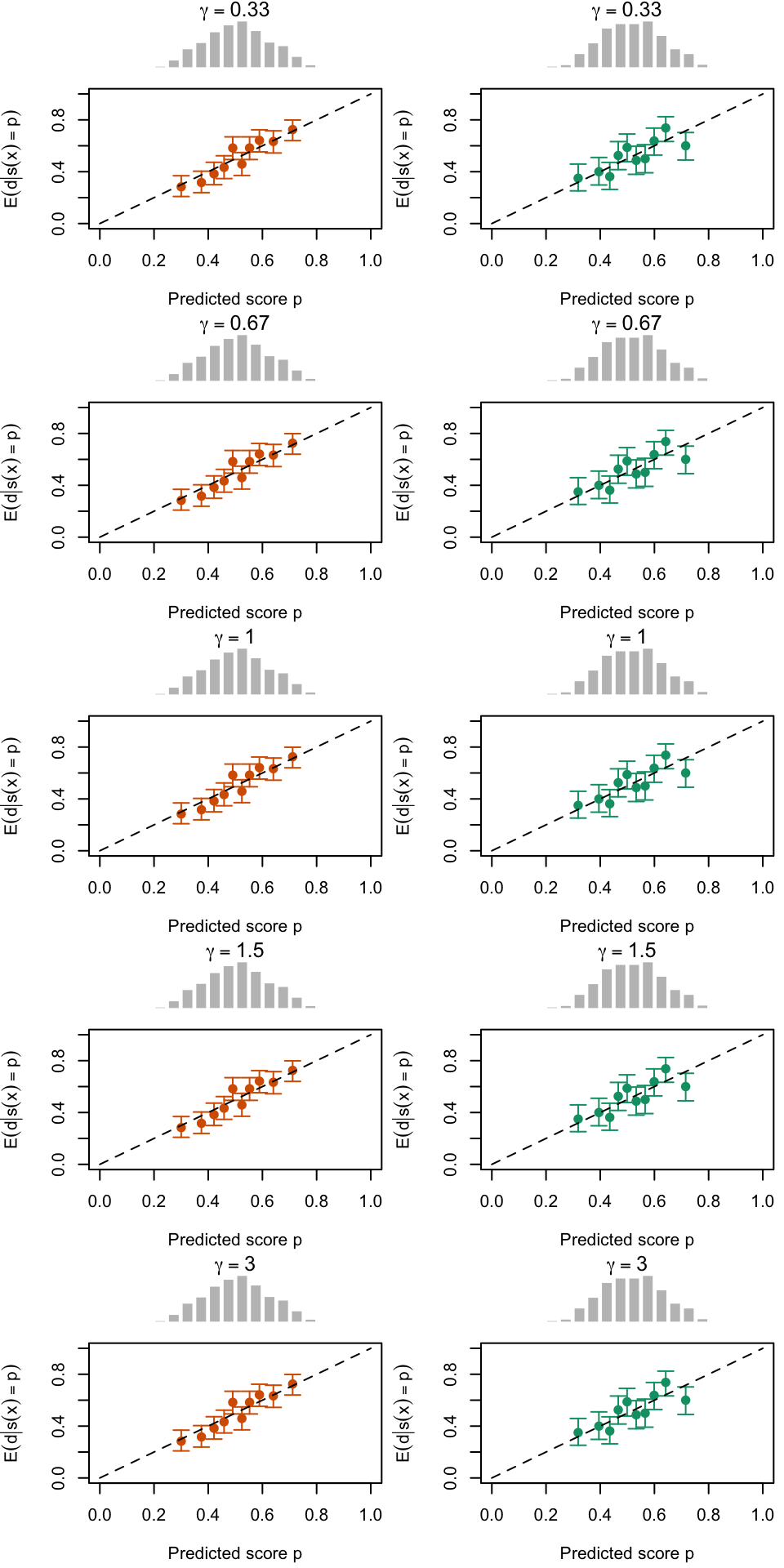
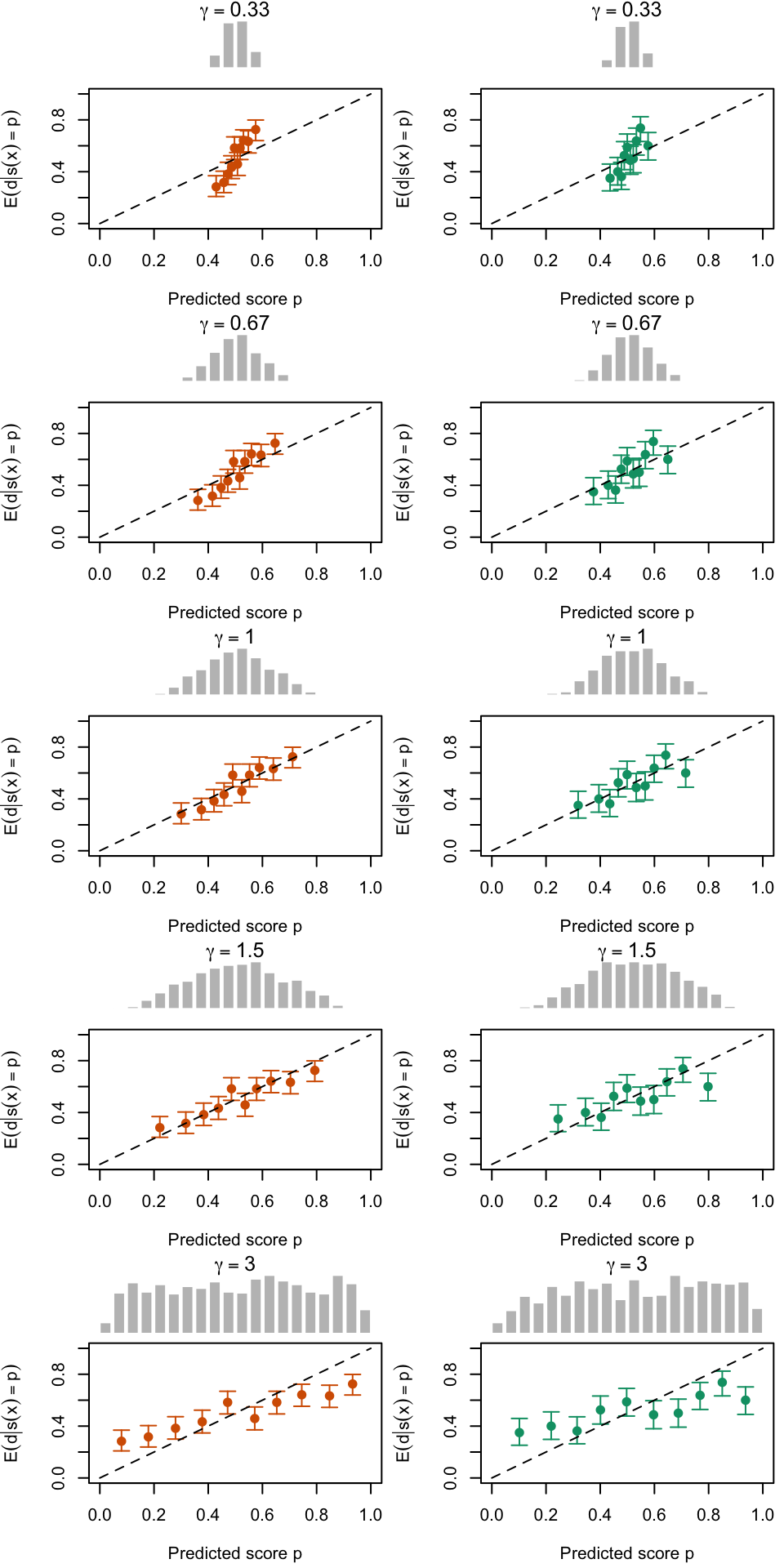
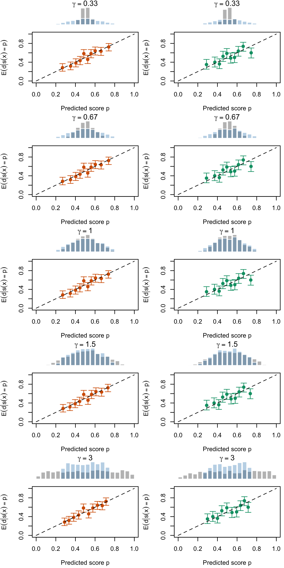
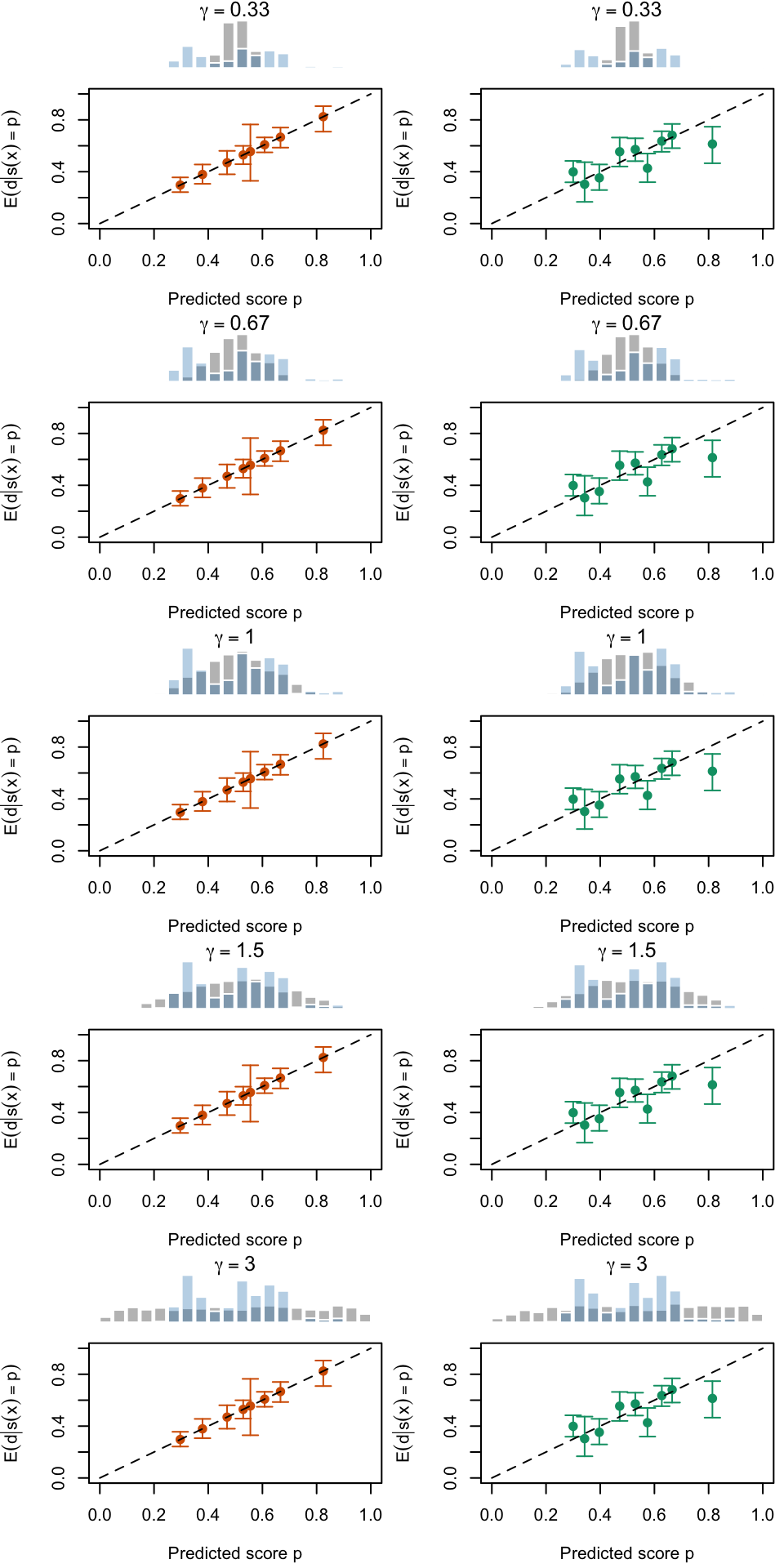
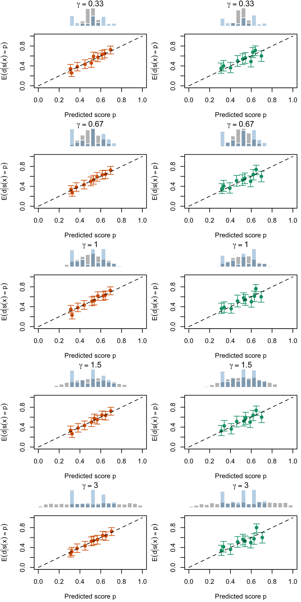
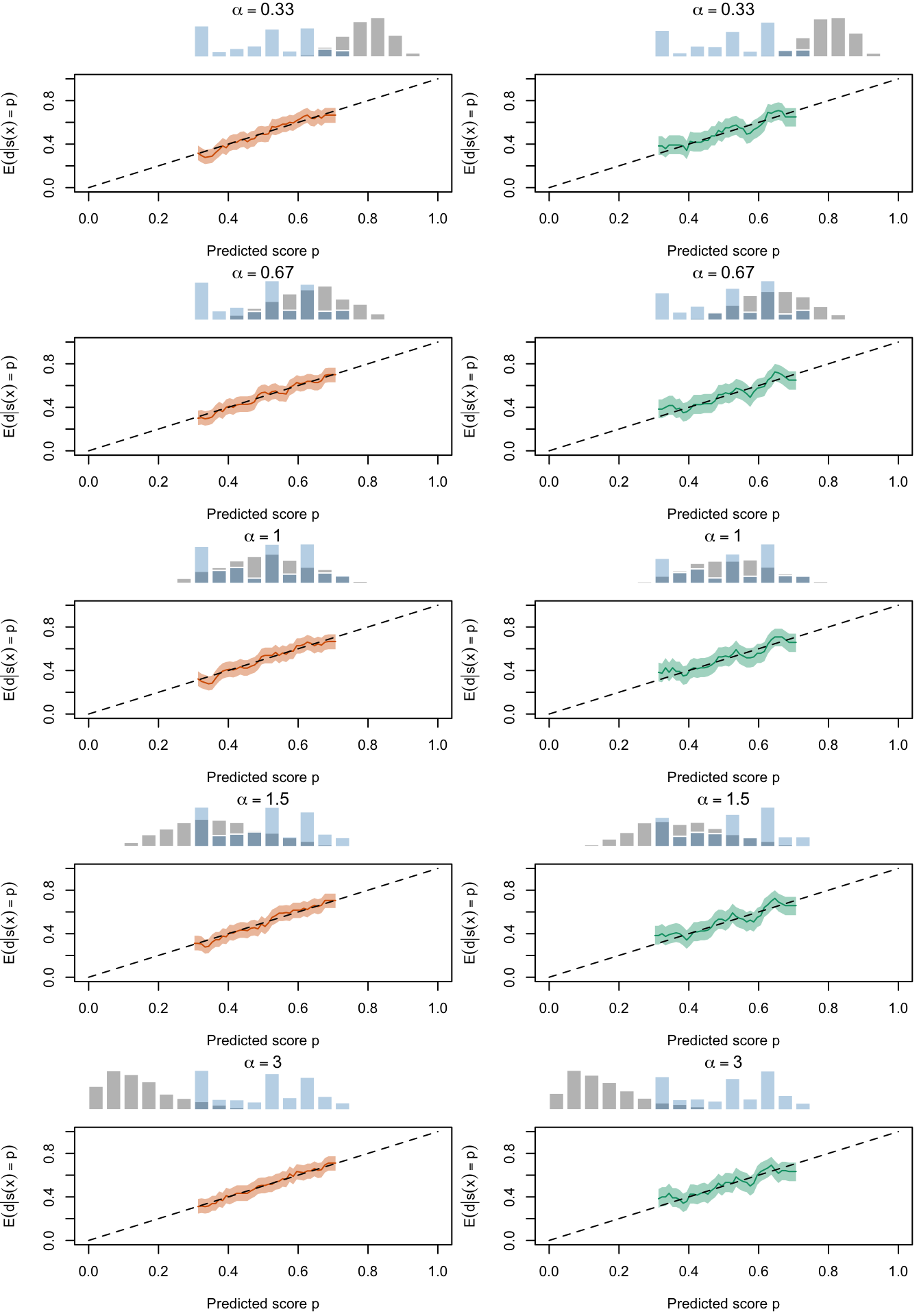
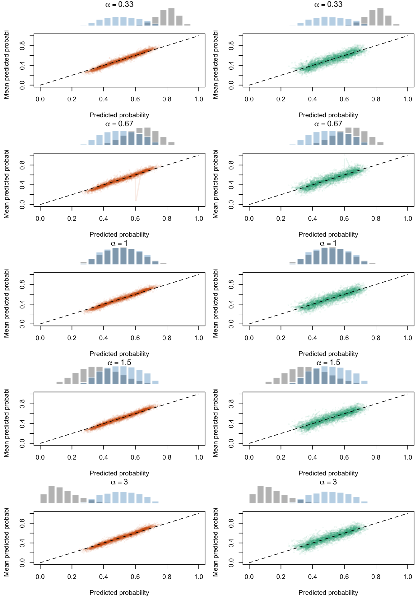
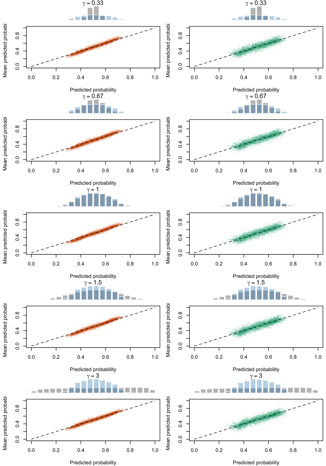
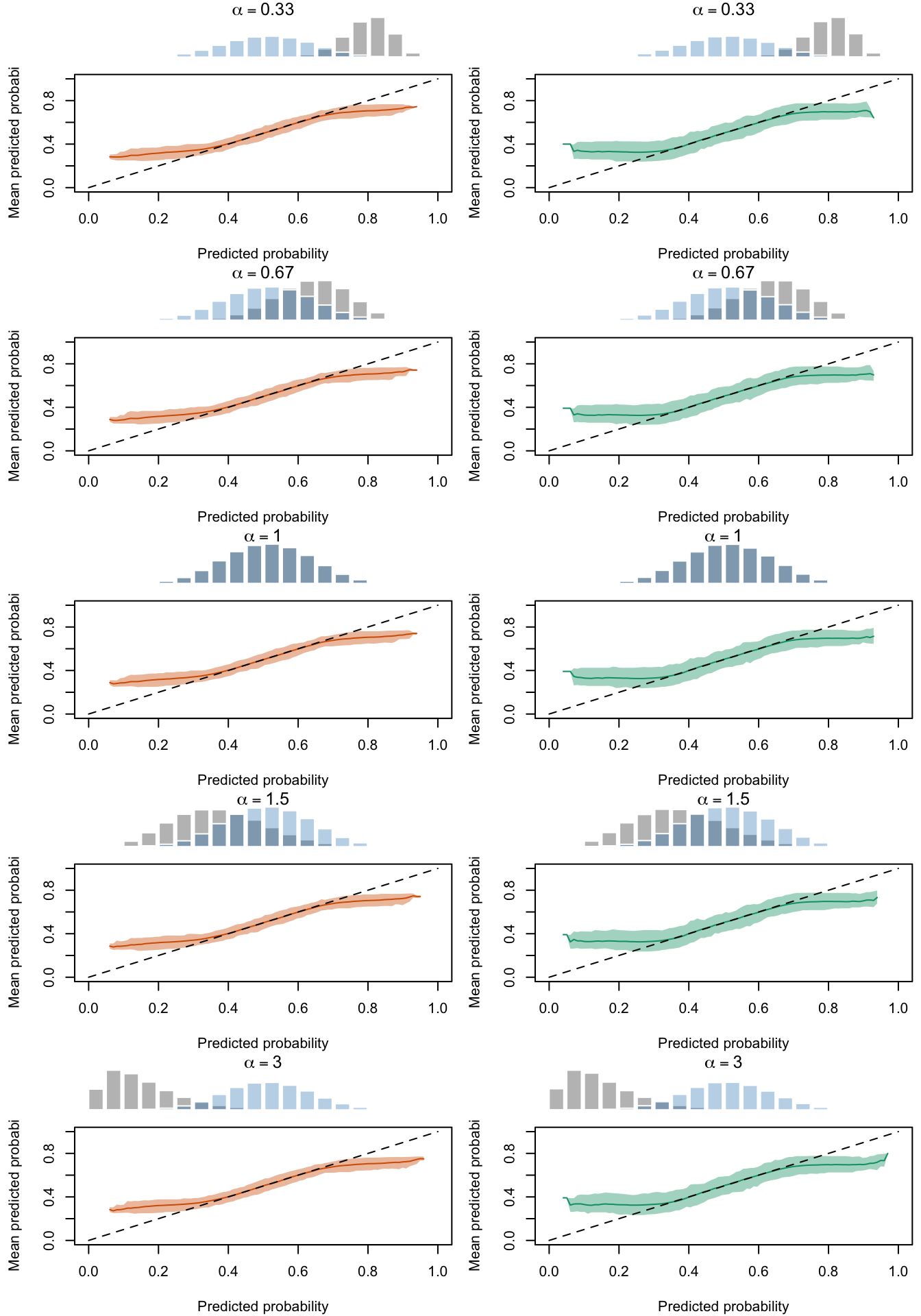
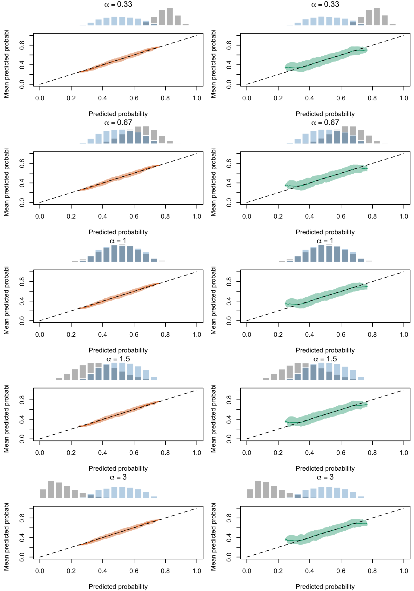
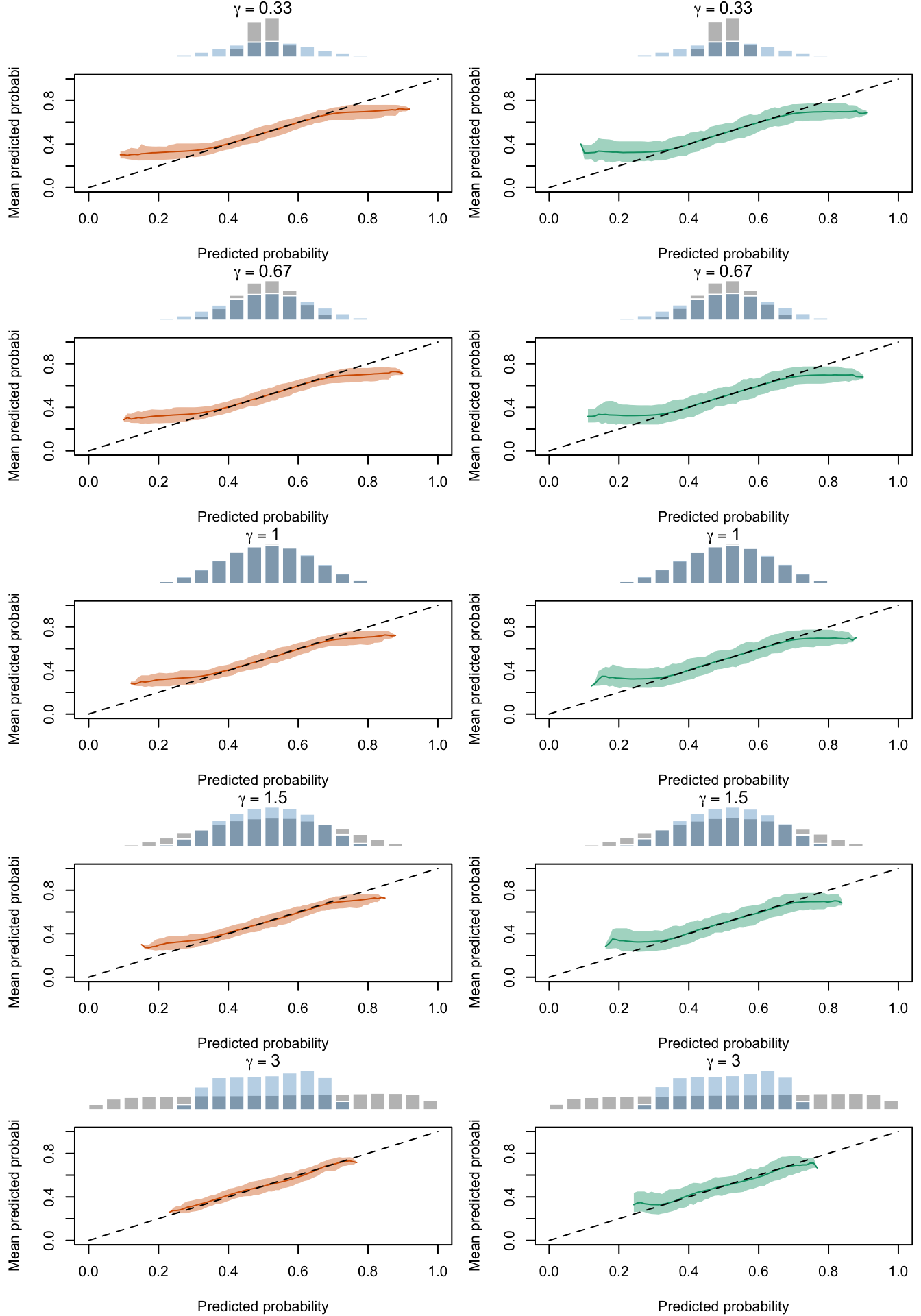
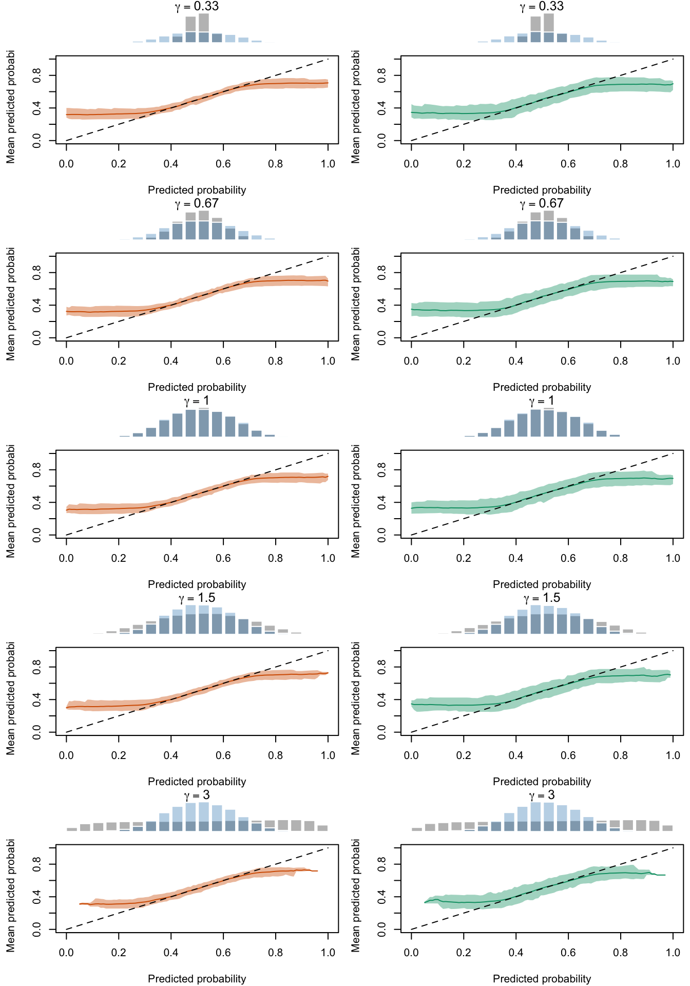
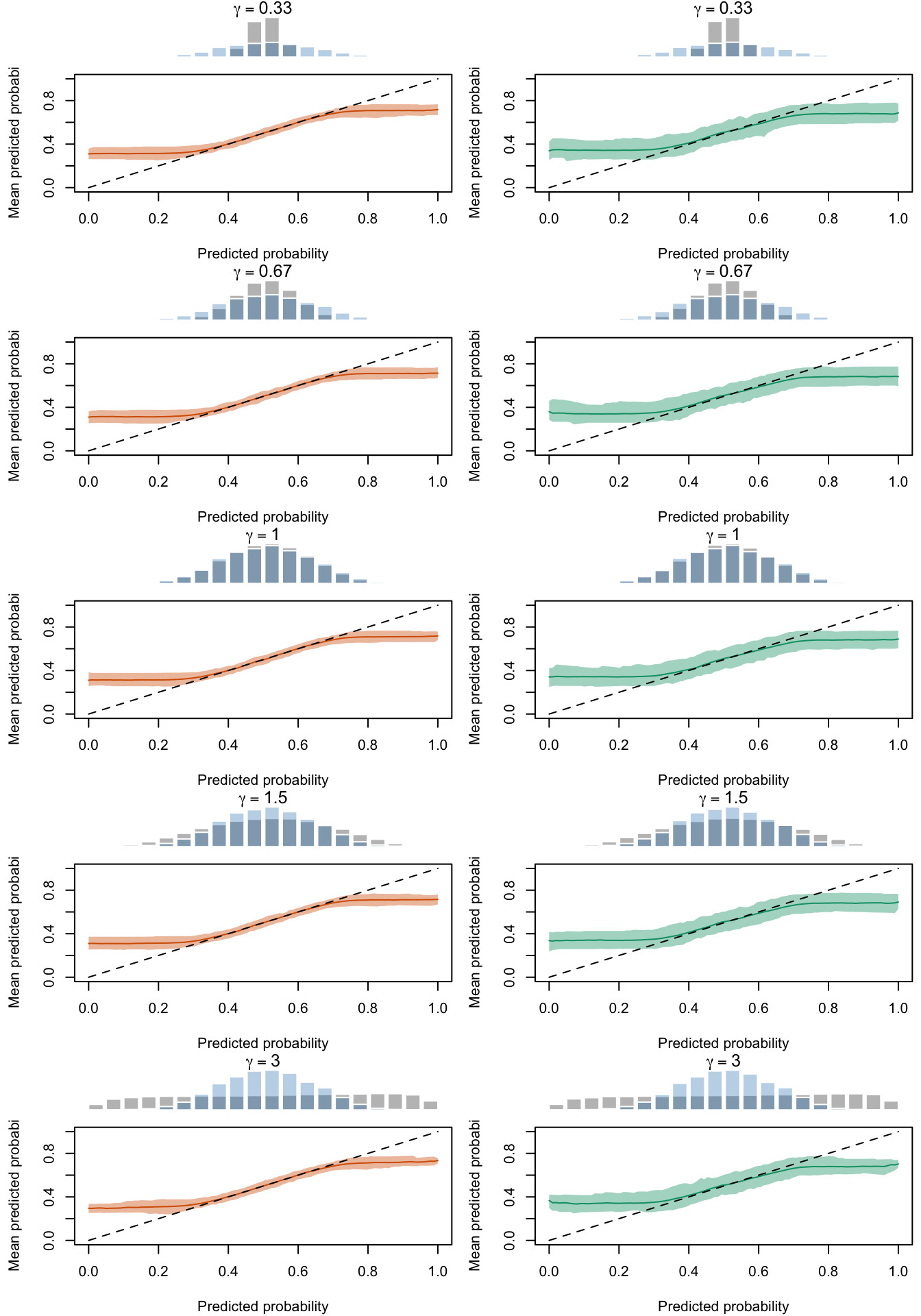
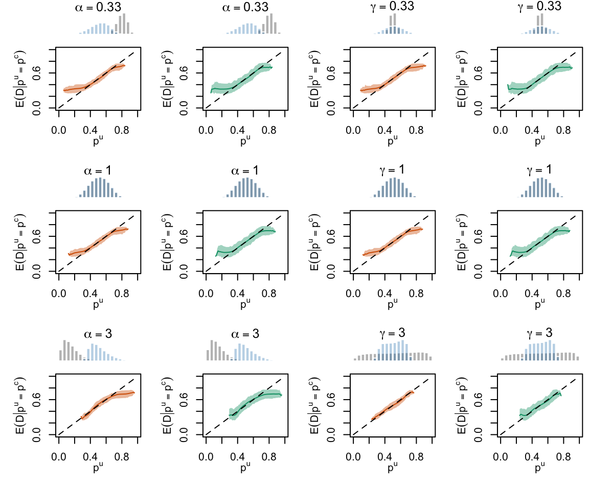
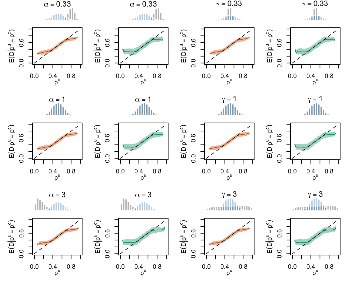
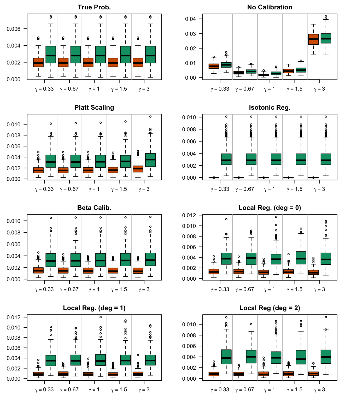
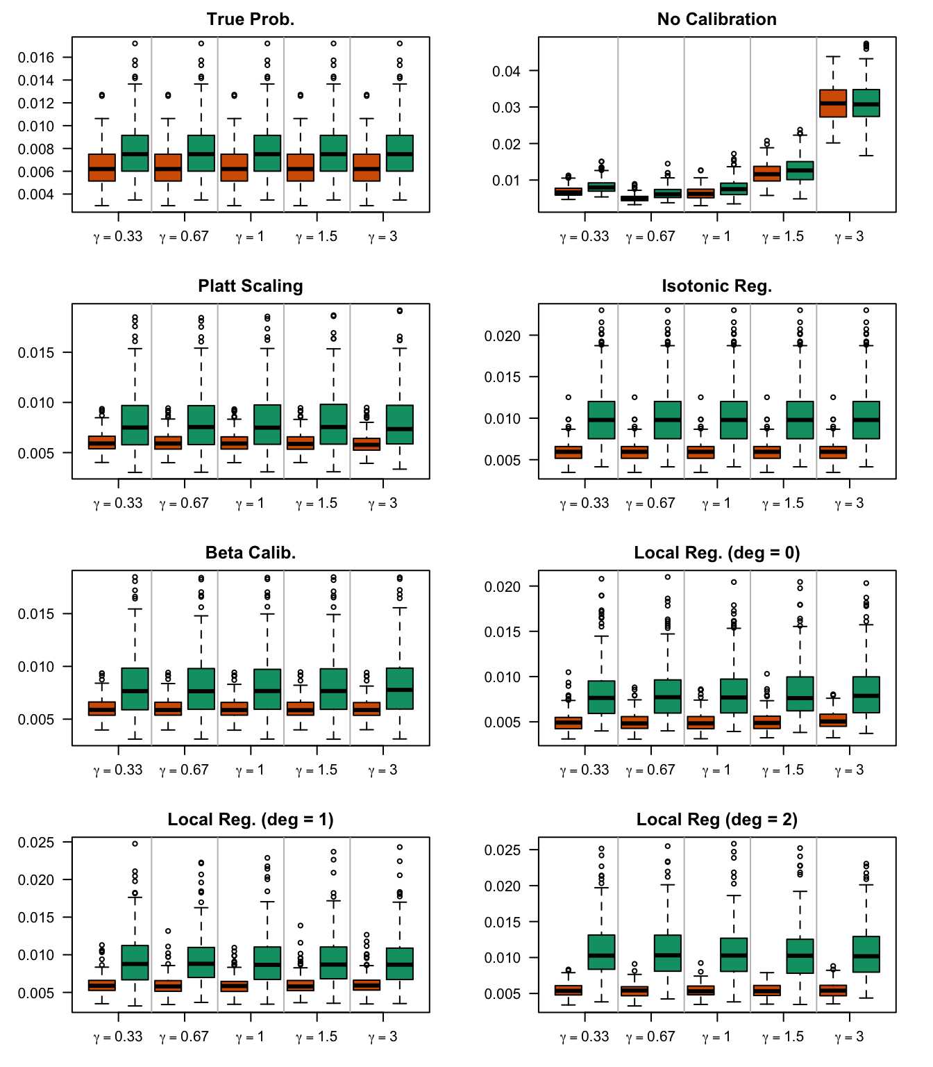
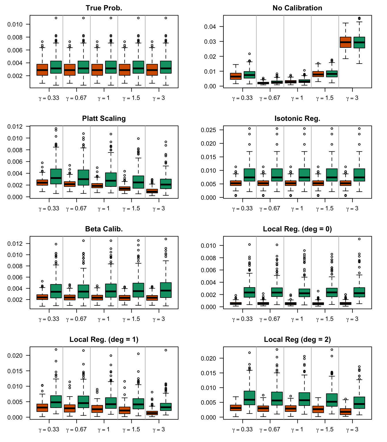
The figures below show a panel of graphs with the superimposed calibration curves obtained with the quantile-based bins. Each tab shows the curves for a type of recalibration used. The first two tabs (True Prob. and No Calibration) show the curves obtained using the true probabilities \(p\) and the uncalibrated probabilities \(p^u\), instead of the recalibrated probabilities \(p^c\). Each row of the panel in the Figures corresponds to a value for either \(\alpha\) or \(\gamma\) used to transform \(p\) to get \(p^u\). The left column shows the calibration curve obtained on the calibration set whereas the right column shows the calibration curve obtained on the test set. The average distribution (computed over the 200 simulations) of the uncalibrated scores and of the calibrated scores are shown in the histograms on top of each graph.
Calibration curves obtained with recalibrated scores. The curves are obtained with quantile-defined bins for the calibration set (left) and for the test set (right) for varying values of \(\alpha\) for 200 replication of the simulations. The histogram on top of each graph show the distribution of the uncalibrated scores, and that of the calibrated scores.
Calibration curves obtained with recalibrated scores. The curves are obtained with quantile-defined bins for the calibration set (left) and for the test set (right) for varying values of \(\alpha\) for 200 replication of the simulations. The histogram on top of each graph show the distribution of the uncalibrated scores, and that of the calibrated scores.
Calibration curves obtained with recalibrated scores. The curves are obtained with quantile-defined bins for the calibration set (left) and for the test set (right) for varying values of \(\alpha\) for 200 replication of the simulations. The histogram on top of each graph show the distribution of the uncalibrated scores, and that of the calibrated scores.
Calibration curves obtained with recalibrated scores. The curves are obtained with quantile-defined bins for the calibration set (left) and for the test set (right) for varying values of \(\alpha\) for 200 replication of the simulations. The histogram on top of each graph show the distribution of the uncalibrated scores, and that of the calibrated scores.
Calibration curves obtained with recalibrated scores. The curves are obtained with quantile-defined bins for the calibration set (left) and for the test set (right) for varying values of \(\alpha\) for 200 replication of the simulations. The histogram on top of each graph show the distribution of the uncalibrated scores, and that of the calibrated scores.
Calibration curves obtained with recalibrated scores. The curves are obtained with quantile-defined bins for the calibration set (left) and for the test set (right) for varying values of \(\alpha\) for 200 replication of the simulations. The histogram on top of each graph show the distribution of the uncalibrated scores, and that of the calibrated scores.
Calibration curves obtained with recalibrated scores. The curves are obtained with quantile-defined bins for the calibration set (left) and for the test set (right) for varying values of \(\alpha\) for 200 replication of the simulations. The histogram on top of each graph show the distribution of the uncalibrated scores, and that of the calibrated scores.
Calibration curves obtained with recalibrated scores. The curves are obtained with quantile-defined bins for the calibration set (left) and for the test set (right) for varying values of \(\alpha\) for 200 replication of the simulations. The histogram on top of each graph show the distribution of the uncalibrated scores, and that of the calibrated scores.
Calibration curves obtained with recalibrated scores. The curves are obtained with quantile-defined bins for the calibration set (left) and for the test set (right) for varying values of \(\gamma\) for 200 replication of the simulations. The histogram on top of each graph show the distribution of the uncalibrated scores, and that of the calibrated scores.
Calibration curves obtained with recalibrated scores. The curves are obtained with quantile-defined bins for the calibration set (left) and for the test set (right) for varying values of \(\gamma\) for 200 replication of the simulations. The histogram on top of each graph show the distribution of the uncalibrated scores, and that of the calibrated scores.
Calibration curves obtained with recalibrated scores. The curves are obtained with quantile-defined bins for the calibration set (left) and for the test set (right) for varying values of \(\gamma\) for 200 replication of the simulations. The histogram on top of each graph show the distribution of the uncalibrated scores, and that of the calibrated scores.
Calibration curves obtained with recalibrated scores. The curves are obtained with quantile-defined bins for the calibration set (left) and for the test set (right) for varying values of \(\gamma\) for 200 replication of the simulations. The histogram on top of each graph show the distribution of the uncalibrated scores, and that of the calibrated scores.
Calibration curves obtained with recalibrated scores. The curves are obtained with quantile-defined bins for the calibration set (left) and for the test set (right) for varying values of \(\gamma\) for 200 replication of the simulations. The histogram on top of each graph show the distribution of the uncalibrated scores, and that of the calibrated scores.
Calibration curves obtained with recalibrated scores. The curves are obtained with quantile-defined bins for the calibration set (left) and for the test set (right) for varying values of \(\gamma\) for 200 replication of the simulations. The histogram on top of each graph show the distribution of the uncalibrated scores, and that of the calibrated scores.
Calibration curves obtained with recalibrated scores. The curves are obtained with quantile-defined bins for the calibration set (left) and for the test set (right) for varying values of \(\gamma\) for 200 replication of the simulations. The histogram on top of each graph show the distribution of the uncalibrated scores, and that of the calibrated scores.
Calibration curves obtained with recalibrated scores. The curves are obtained with quantile-defined bins for the calibration set (left) and for the test set (right) for varying values of \(\gamma\) for 200 replication of the simulations. The histogram on top of each graph show the distribution of the uncalibrated scores, and that of the calibrated scores.
Let us visualize the calibration curves in another way.
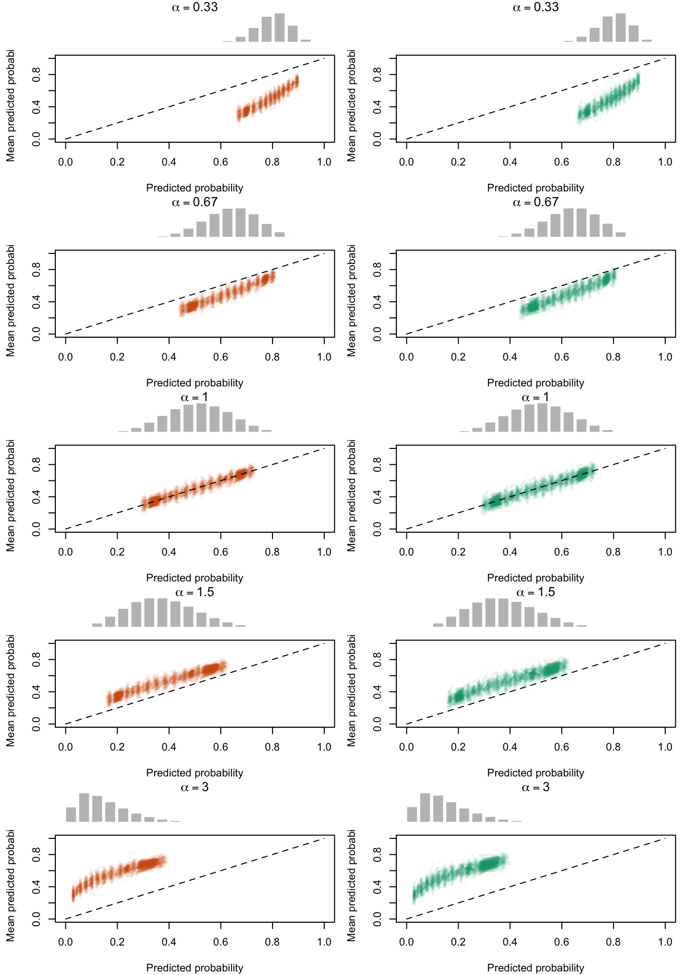
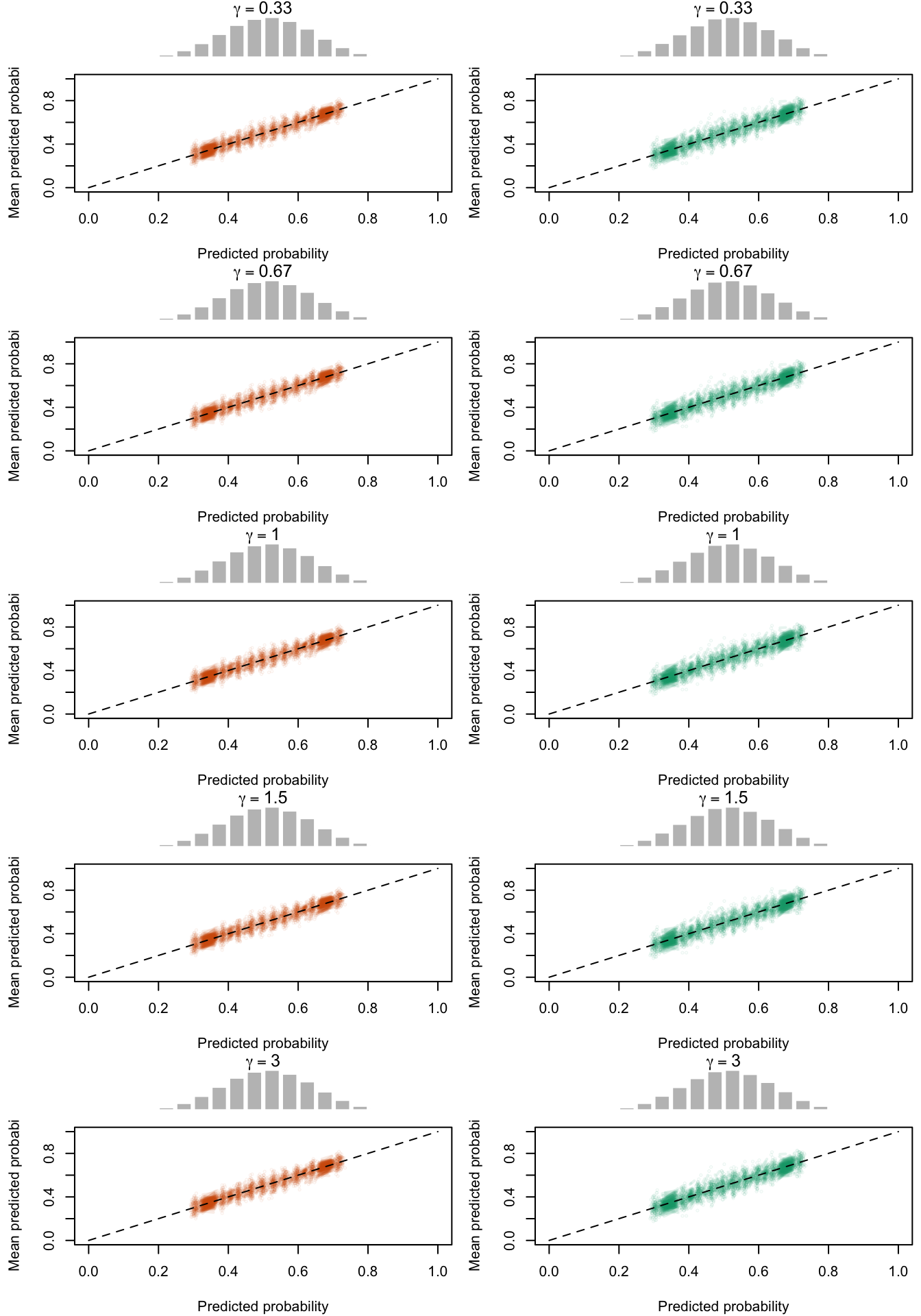
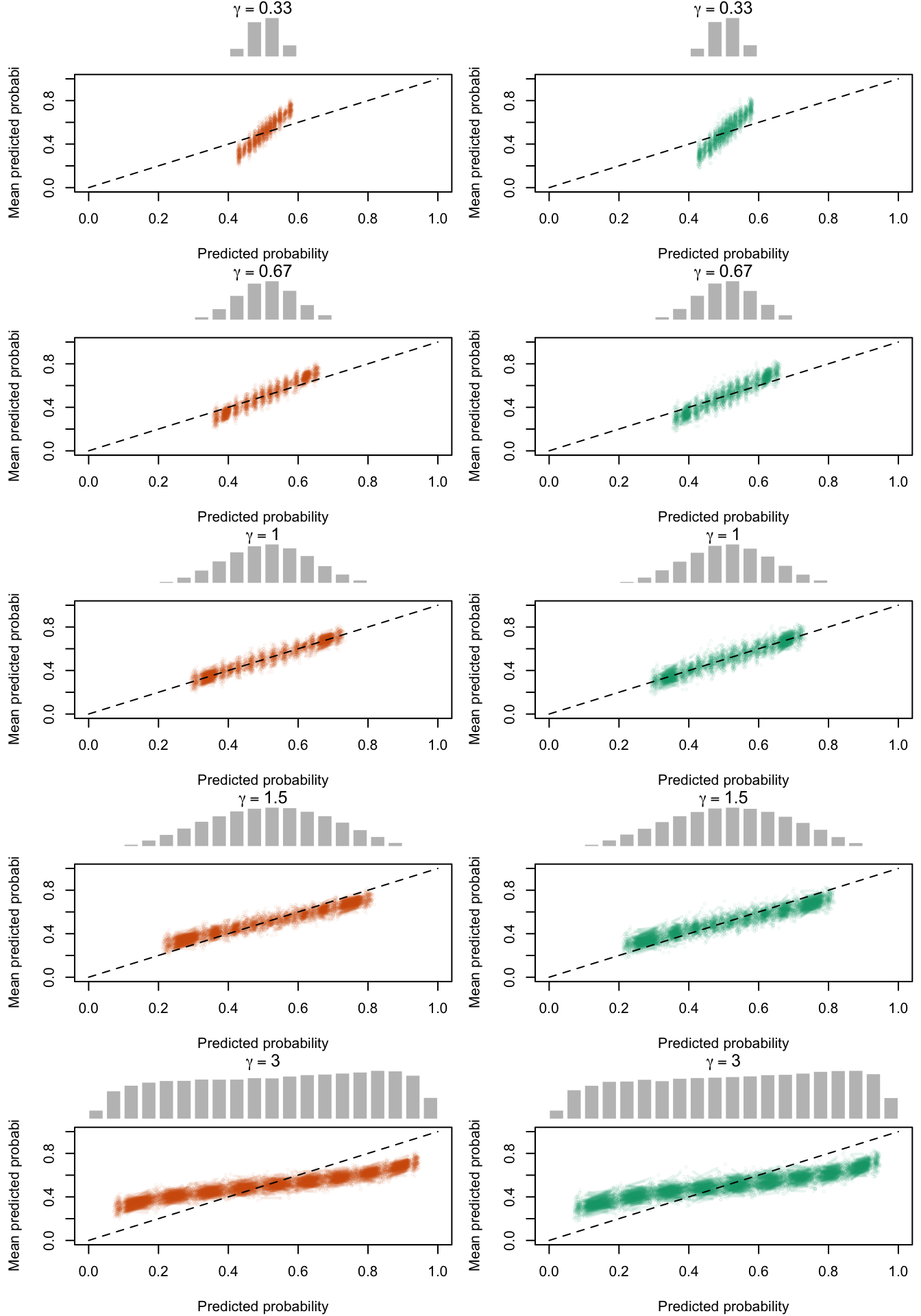
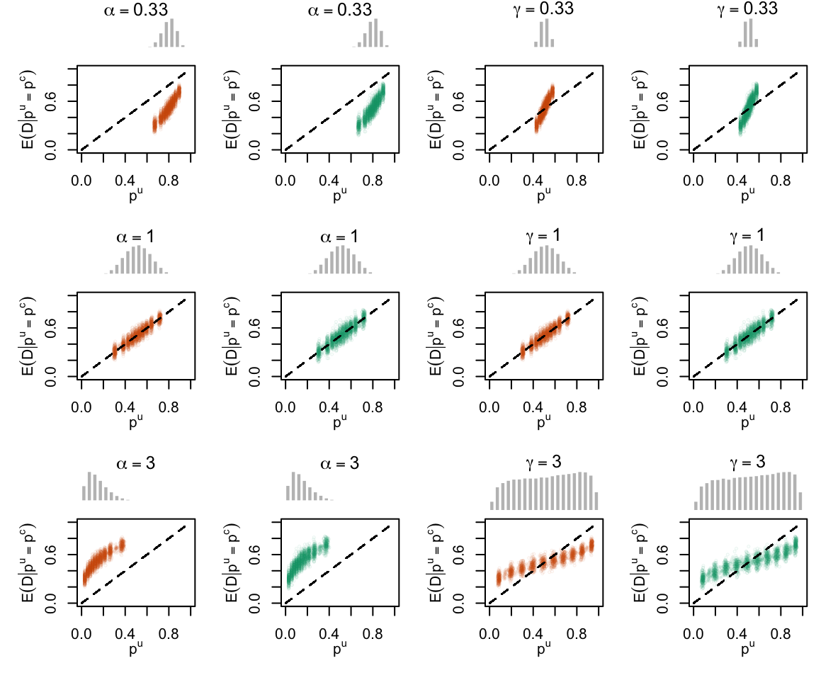
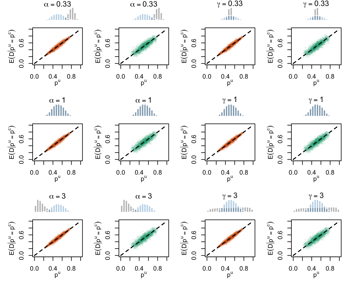
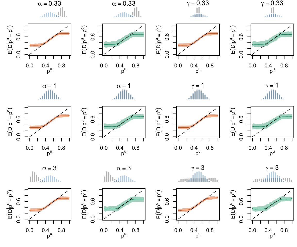
Figure 2.19: Calibration Curves Calculated with True Probabilities as the Scores. The curves are obtained with quantile binning, for the calibration set (orange) and for the test set (green) for varying values of \(\alpha\) and \(\gamma\). The curves of the 200 replications of the simulations are superimposed. The histogram on top of each graph show the distribution of the true probabilities
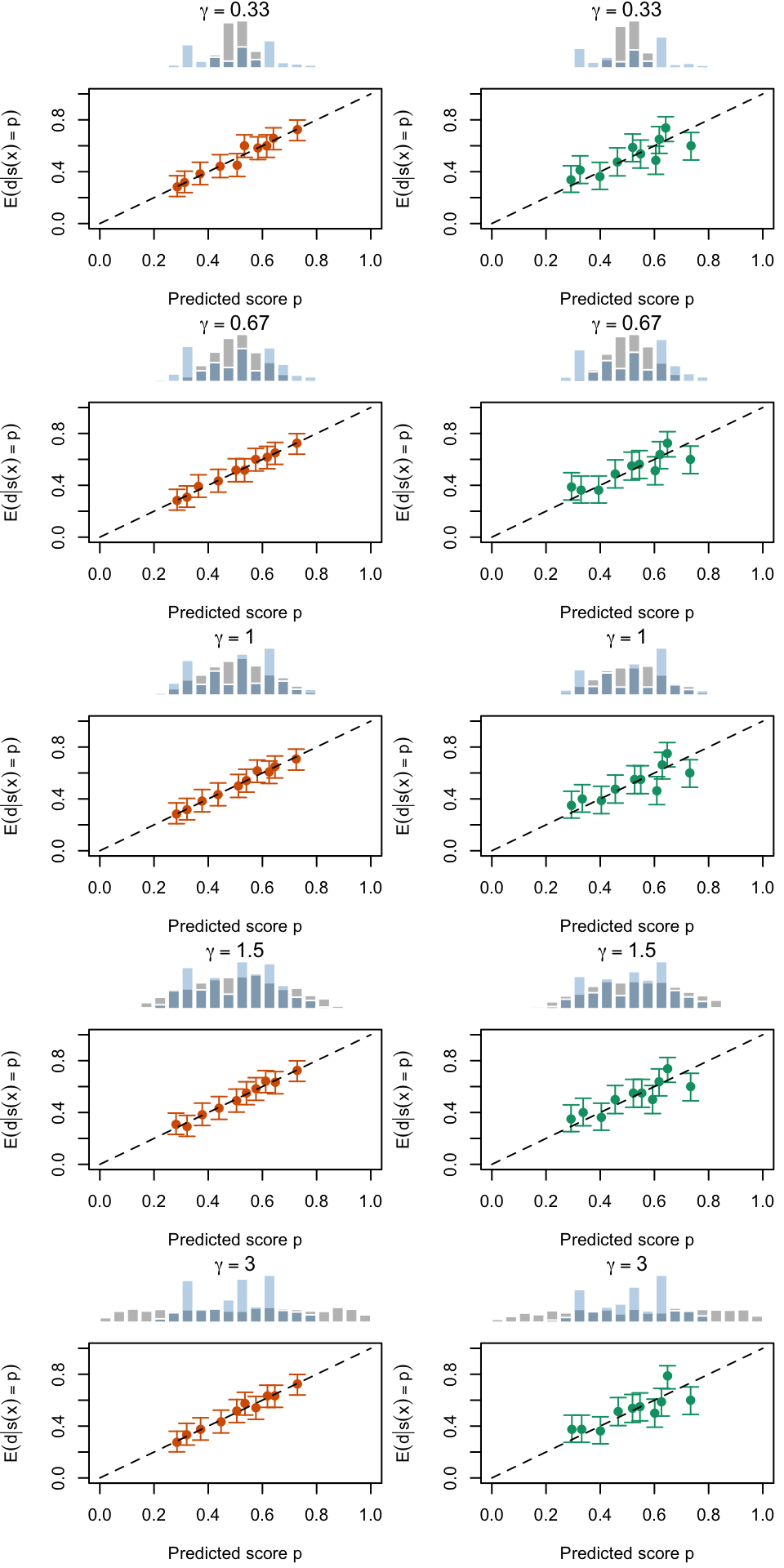
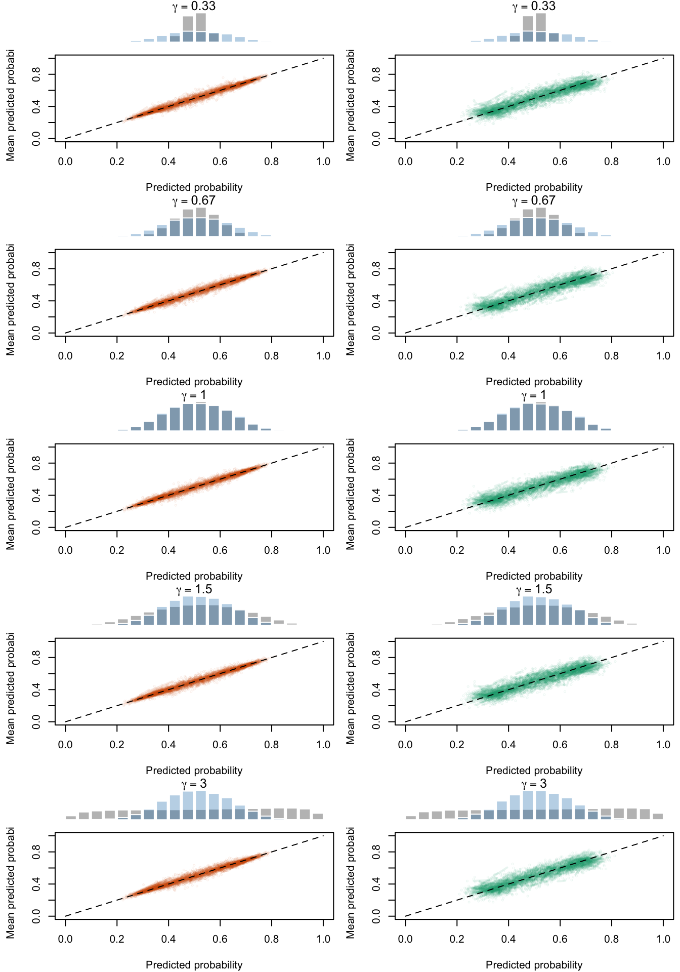
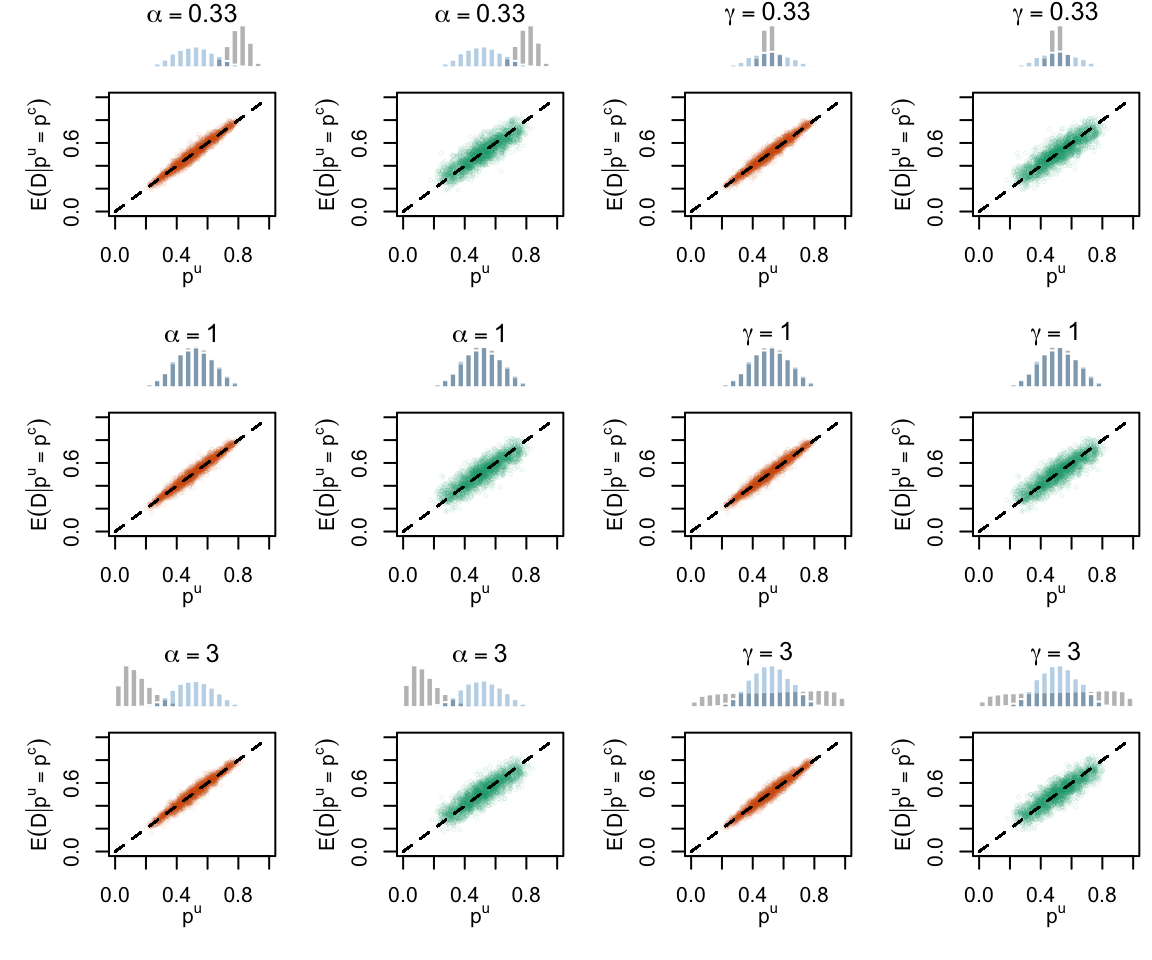
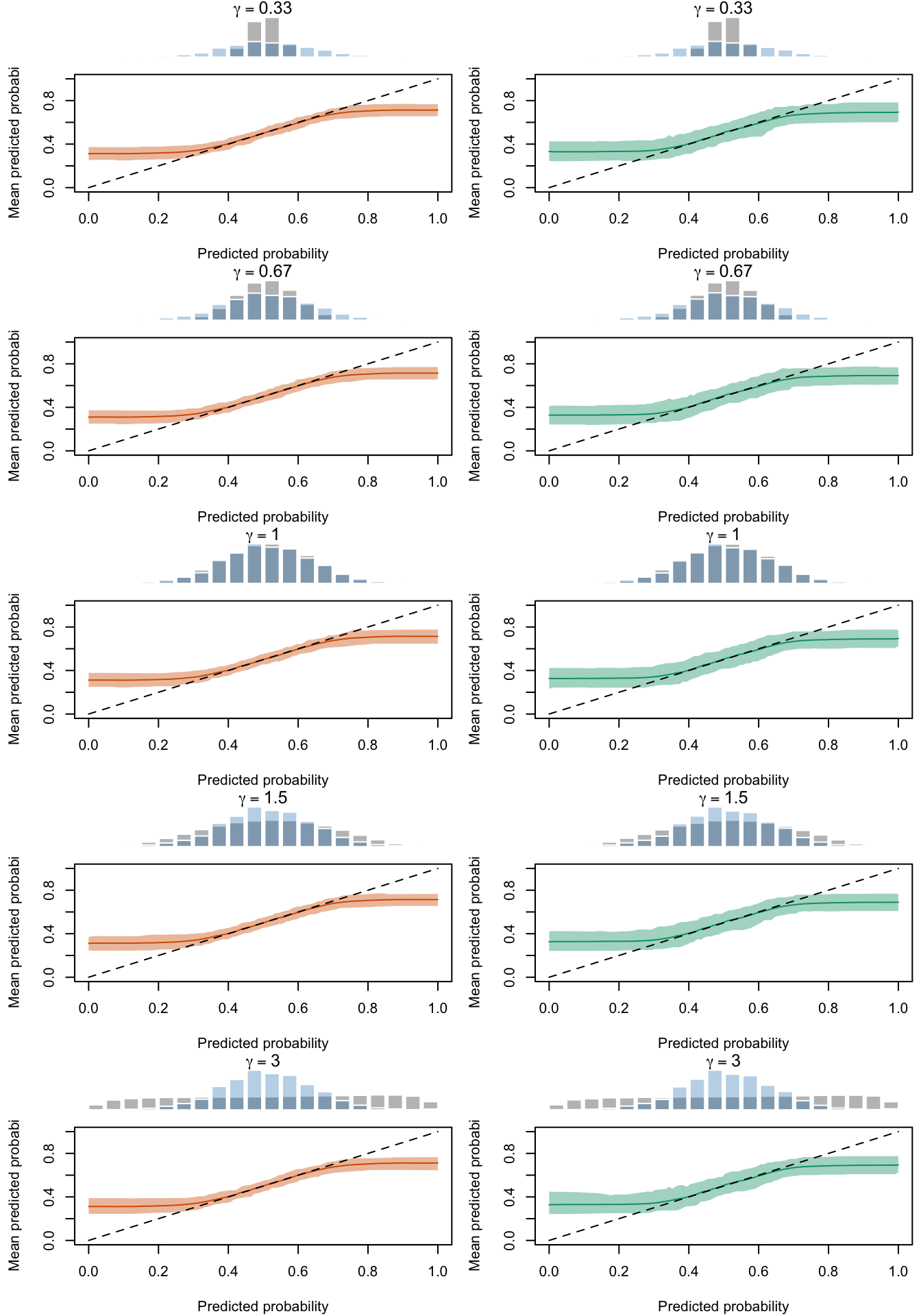
Figure 2.20: Calibration Curves Calculated with Uncalibrated Scores. The curves are obtained with quantile binning, for the calibration set (orange) and for the test set (green) for varying values of \(\alpha\) and \(\gamma\). The curves of the 200 replications of the simulations are superimposed. The histogram on top of each graph show the distribution of the true probabilities.
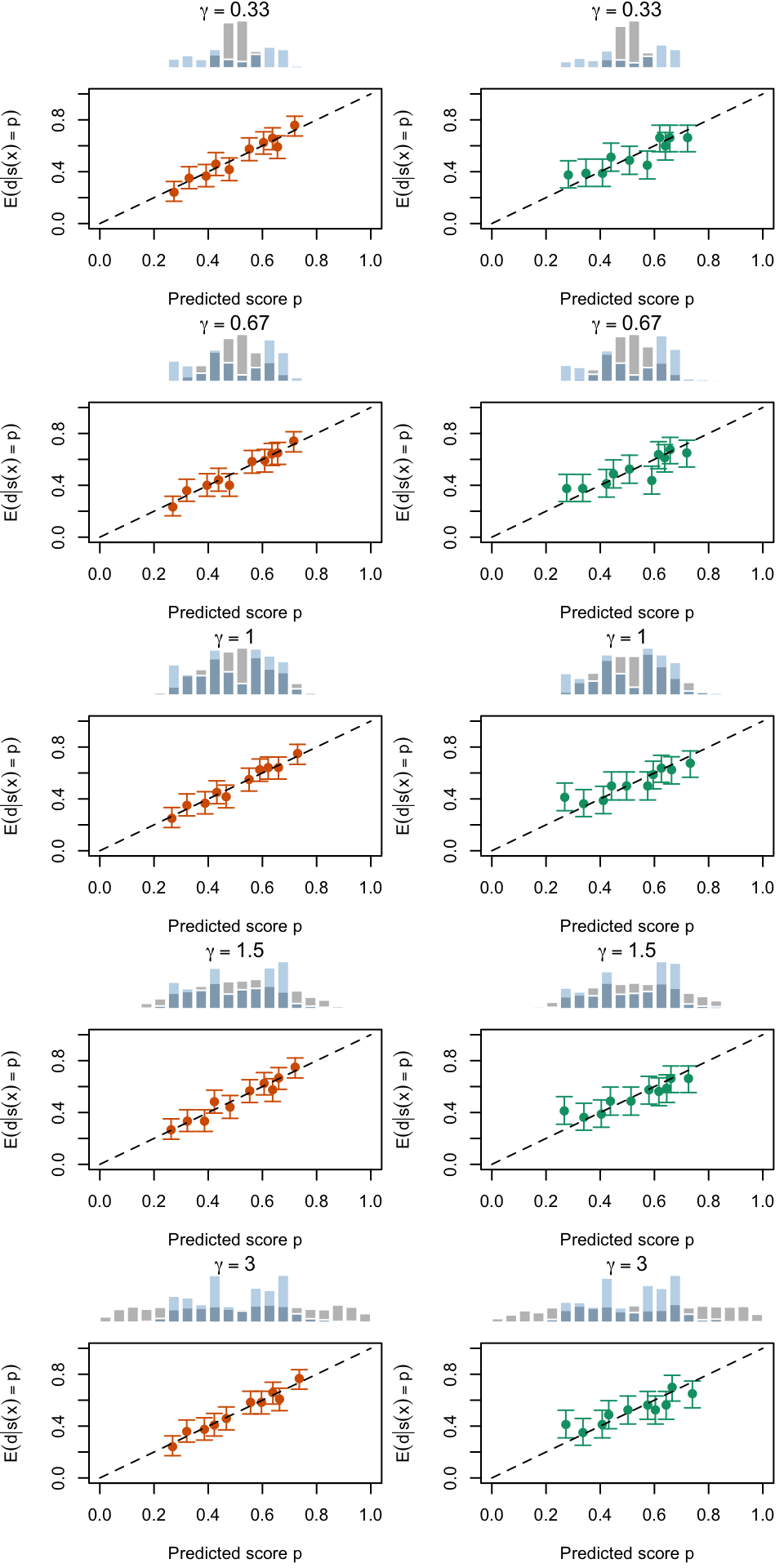
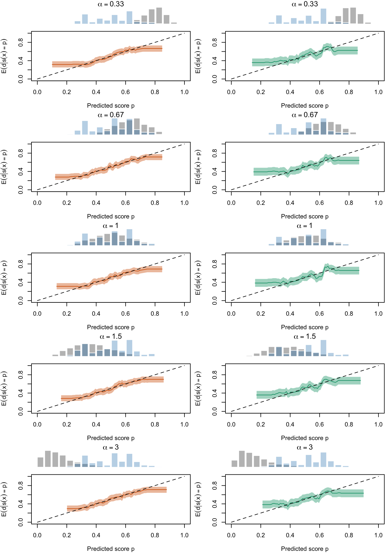
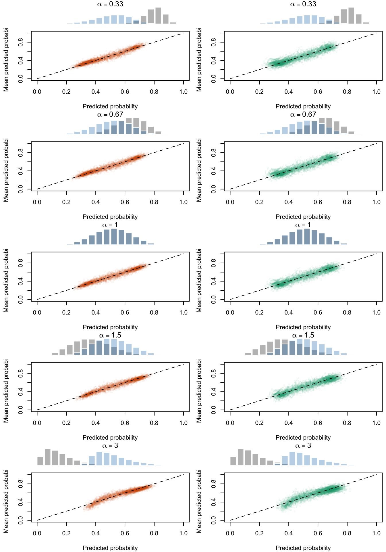
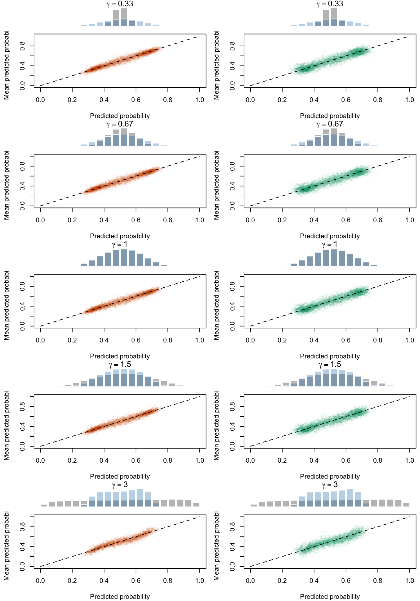
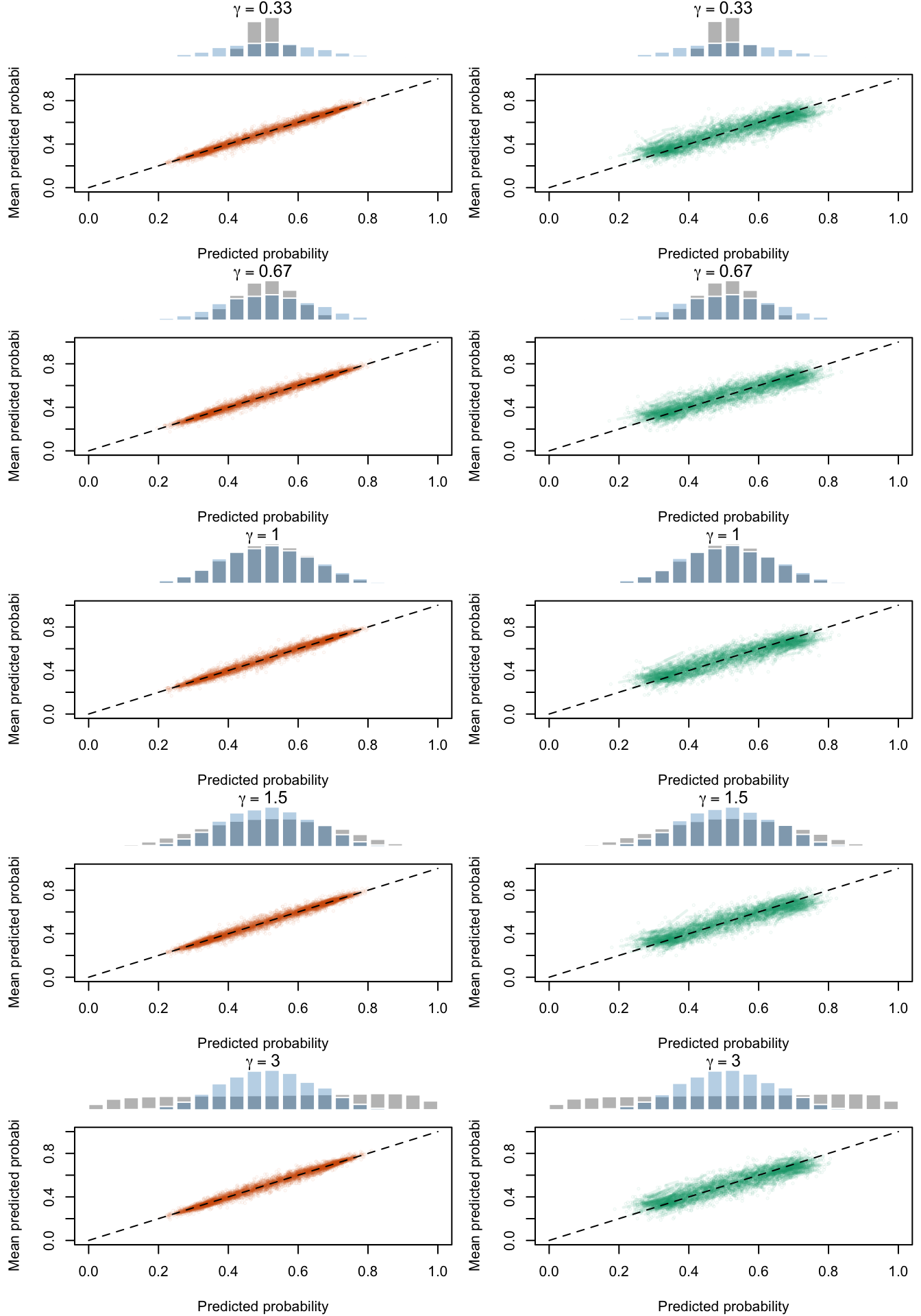
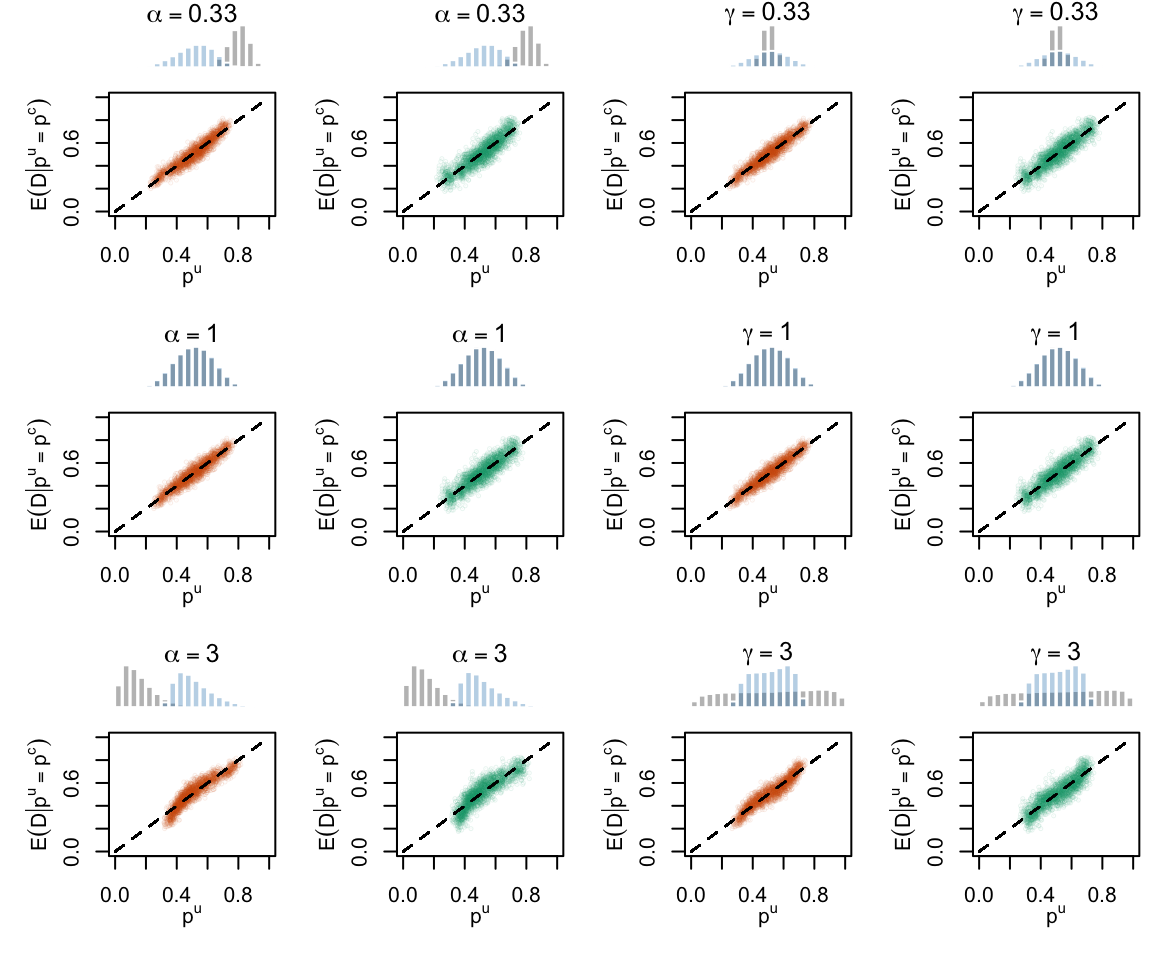
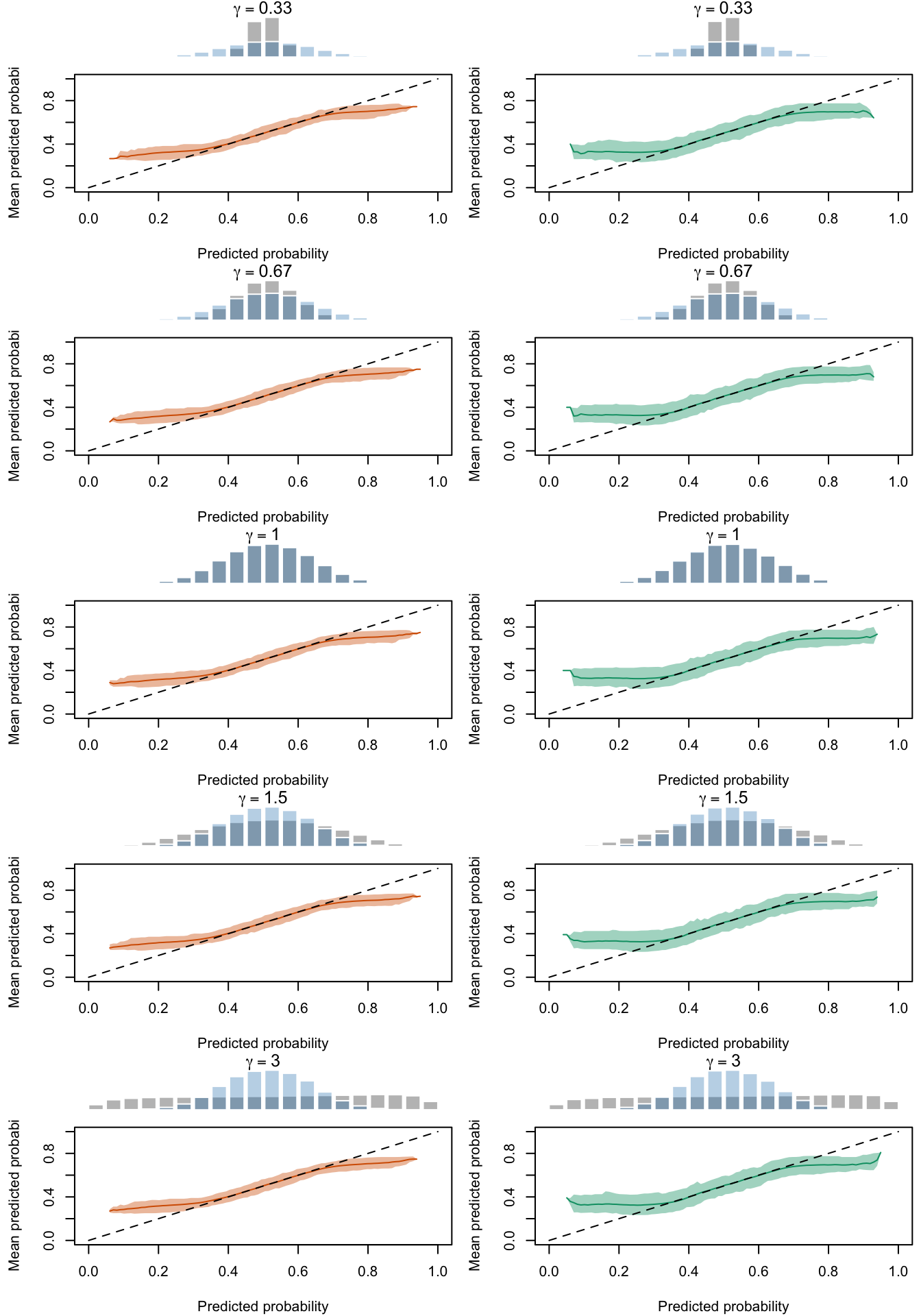
Figure 2.21: Calibration Curves Calculated with Scores Recalibrated Using Platt Scaling. The curves are obtained with quantile binning, for the calibration set (orange) and for the test set (green) for varying values of \(\alpha\) and \(\gamma\). The curves of the 200 replications of the simulations are superimposed. The histogram on top of each graph show the distribution of the uncalibrated scores (gray), and that of the calibrated scores (blue).
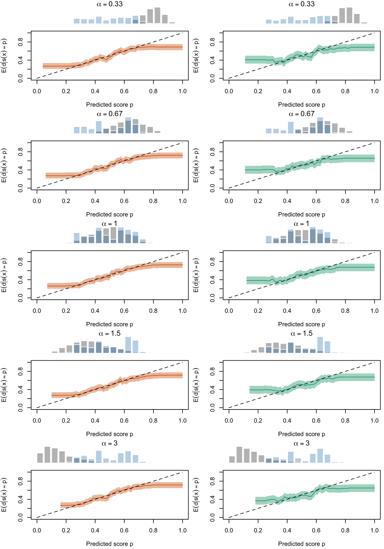
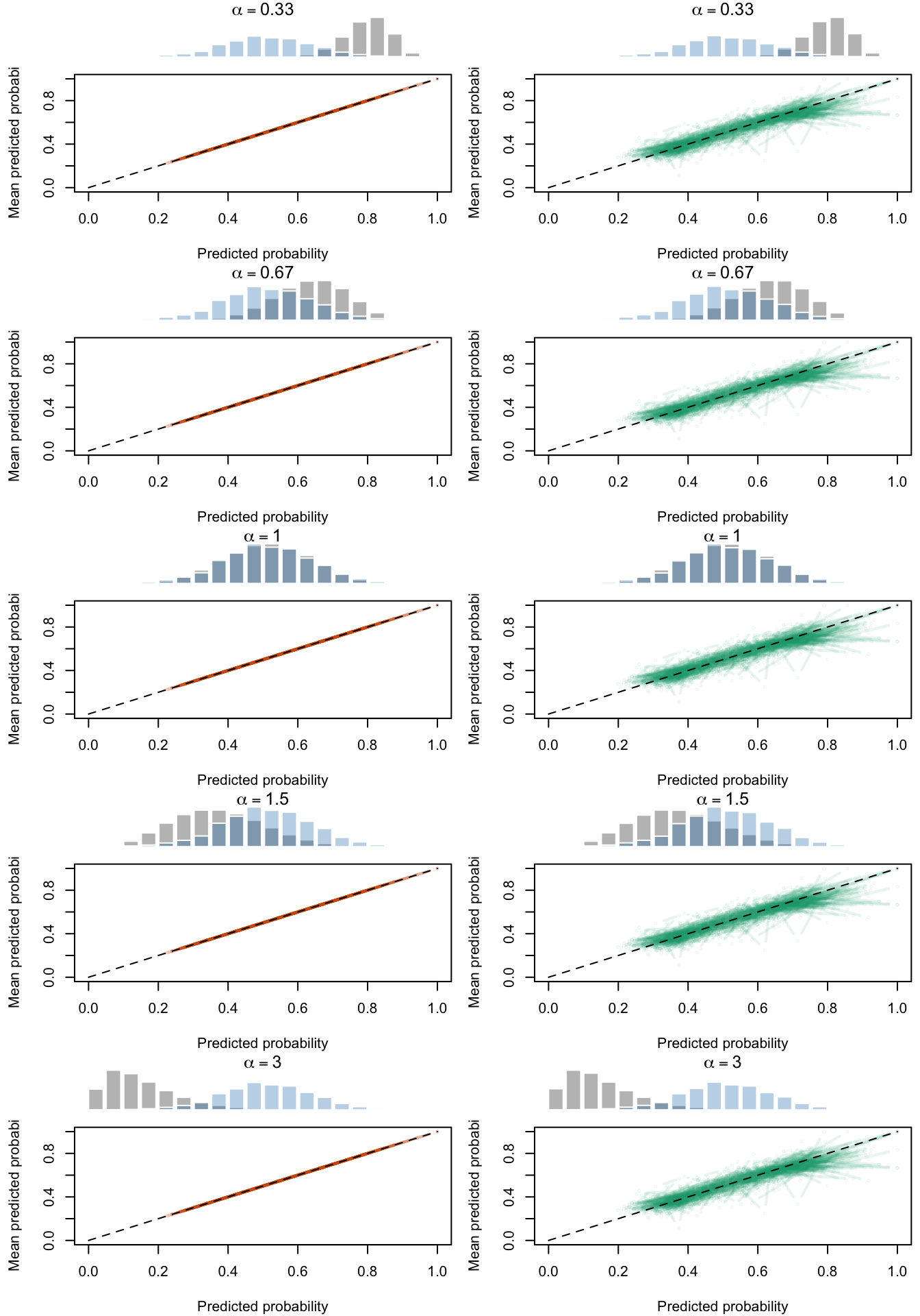
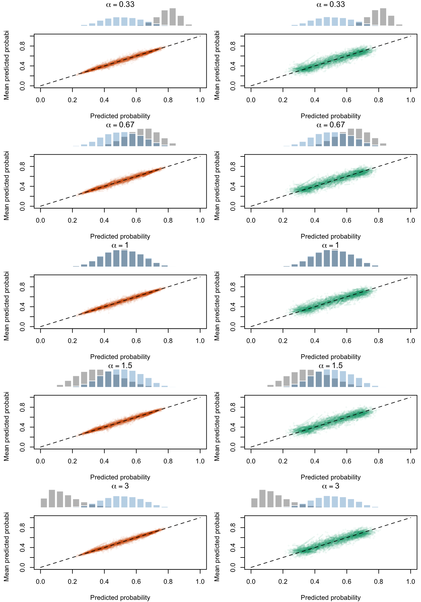
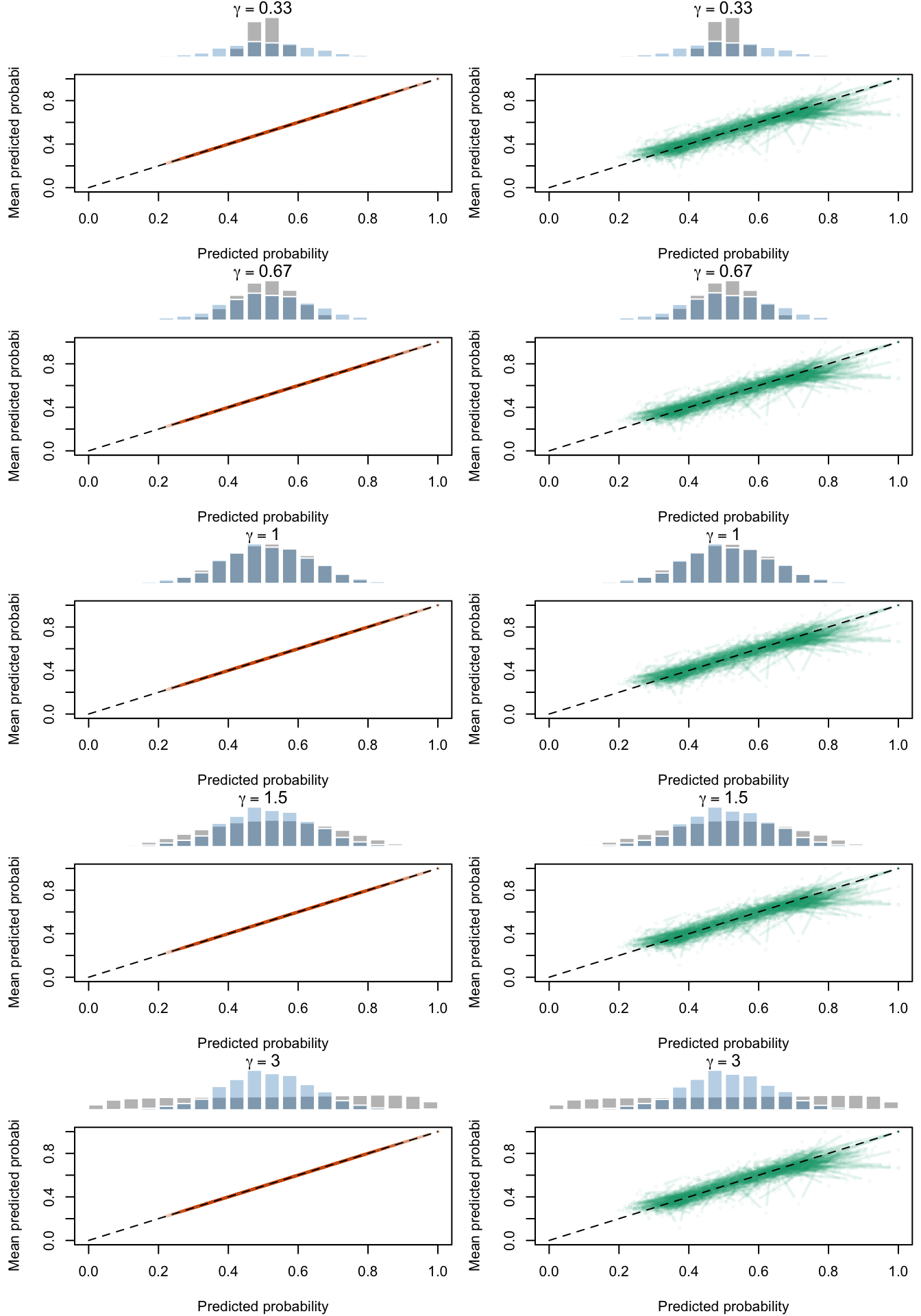
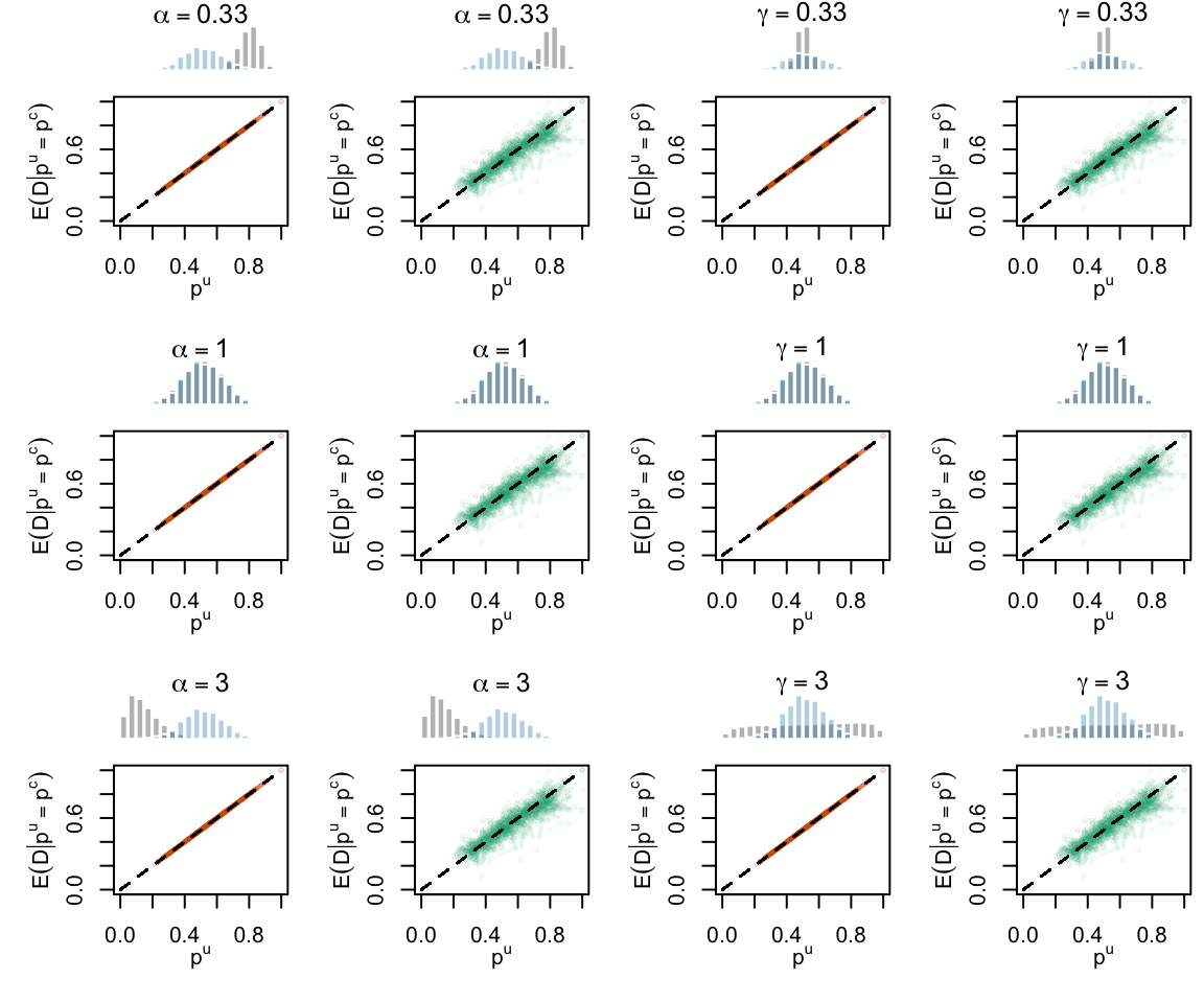
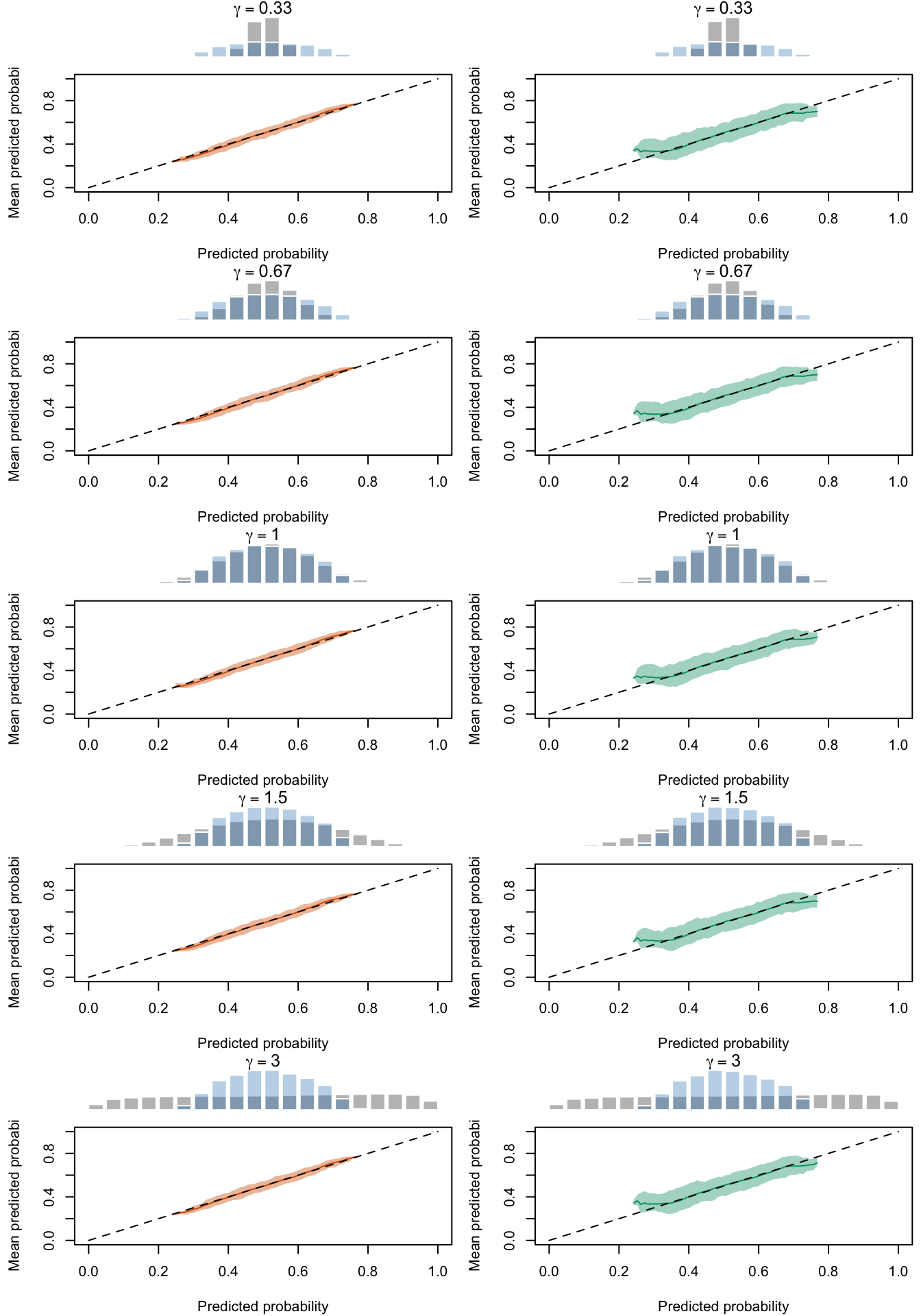
Figure 2.22: Calibration Curves Calculated with Scores Recalibrated Using Isotonic Regression. The curves are obtained with quantile binning, for the calibration set (orange) and for the test set (green) for varying values of \(\alpha\) and \(\gamma\). The curves of the 200 replications of the simulations are superimposed. The histogram on top of each graph show the distribution of the uncalibrated scores (gray), and that of the calibrated scores (blue).
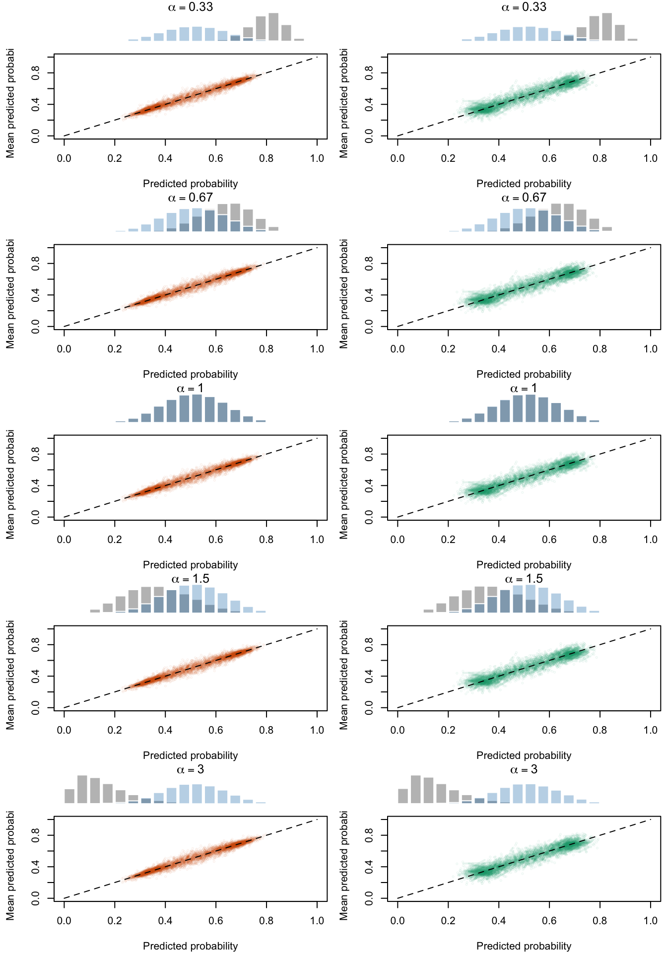
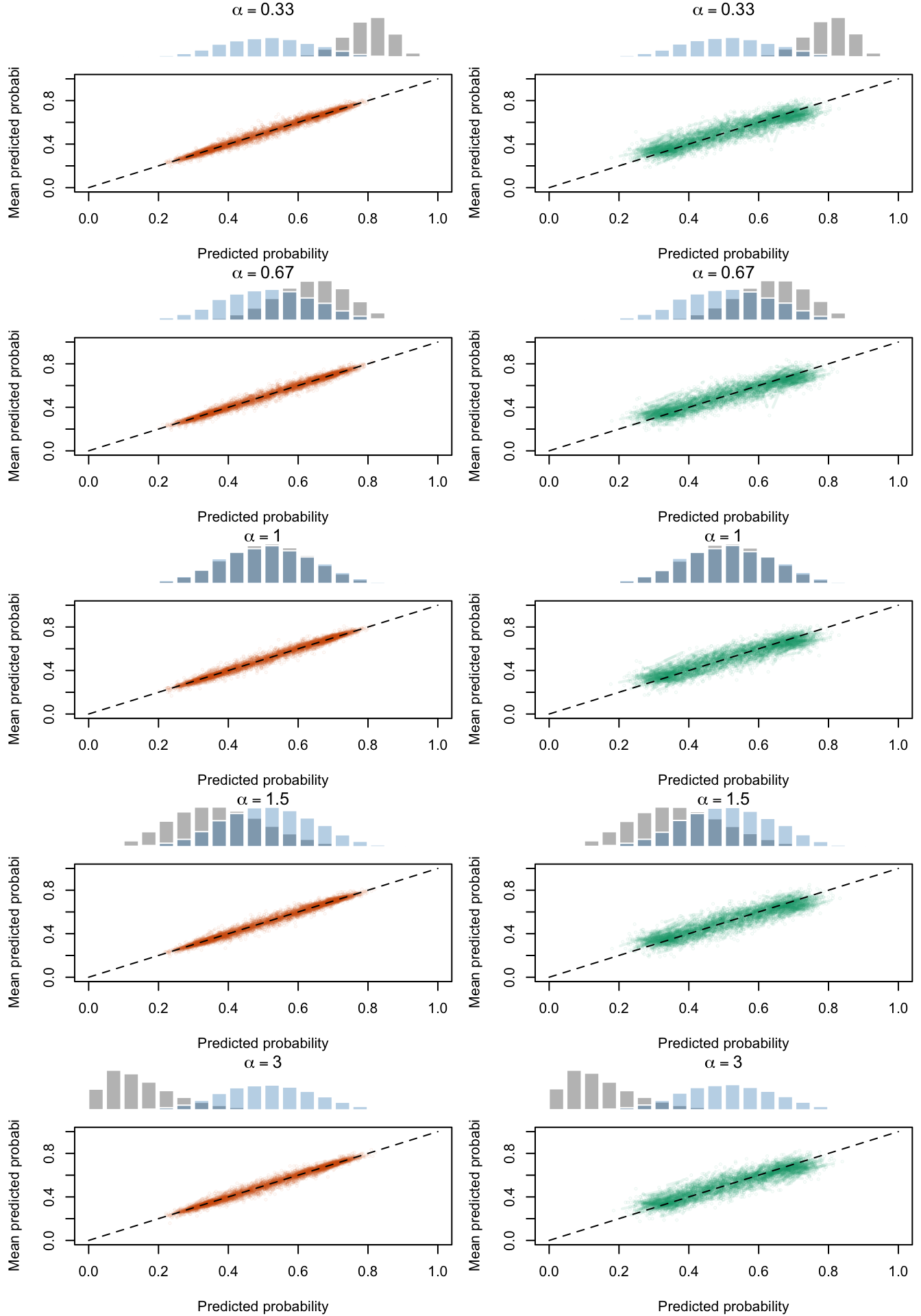
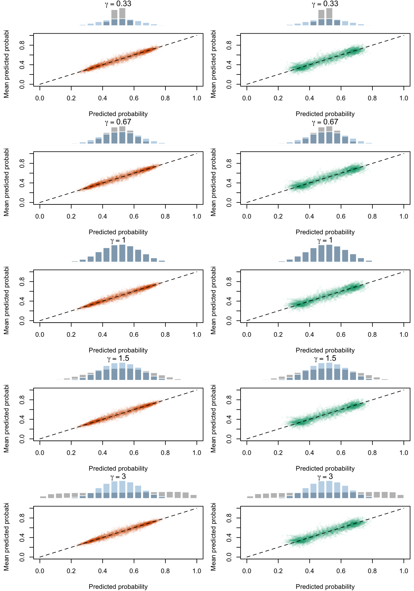
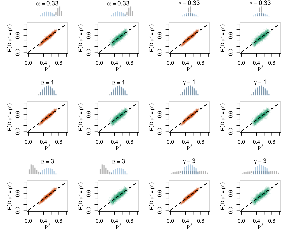
Figure 2.23: Calibration Curves Calculated with Scores Recalibrated Using Beta Calibration. The curves are obtained with quantile binning, for the calibration set (orange) and for the test set (green) for varying values of \(\alpha\) and \(\gamma\). The curves of the 200 replications of the simulations are superimposed. The histogram on top of each graph show the distribution of the uncalibrated scores (gray), and that of the calibrated scores (blue).
Figure 2.24: Calibration Curves Calculated with Scores Recalibrated Using Local Regression (with degree 0). The curves are obtained with quantile binning, for the calibration set (orange) and for the test set (green) for varying values of \(\alpha\) and \(\gamma\). The curves of the 200 replications of the simulations are superimposed. The histogram on top of each graph show the distribution of the uncalibrated scores (gray), and that of the calibrated scores (blue).
Figure 2.25: Calibration Curves Calculated with Scores Recalibrated Using Local Regression (with degree 1). The curves are obtained with quantile binning, for the calibration set (orange) and for the test set (green) for varying values of \(\alpha\) and \(\gamma\). The curves of the 200 replications of the simulations are superimposed. The histogram on top of each graph show the distribution of the uncalibrated scores (gray), and that of the calibrated scores (blue).
Figure 2.26: Calibration Curves Calculated with Scores Recalibrated Using Local Regression (with degree 2). The curves are obtained with quantile binning, for the calibration set (orange) and for the test set (green) for varying values of \(\alpha\) and \(\gamma\). The curves of the 200 replications of the simulations are superimposed. The histogram on top of each graph show the distribution of the uncalibrated scores (gray), and that of the calibrated scores (blue).
2.7.2 Calibration Curve with Local Regression
We will plot the calibration curves estimated using the local regression method, for all type of transformation of the probabilities made (varying either \(\alpha\) or \(\gamma\)).
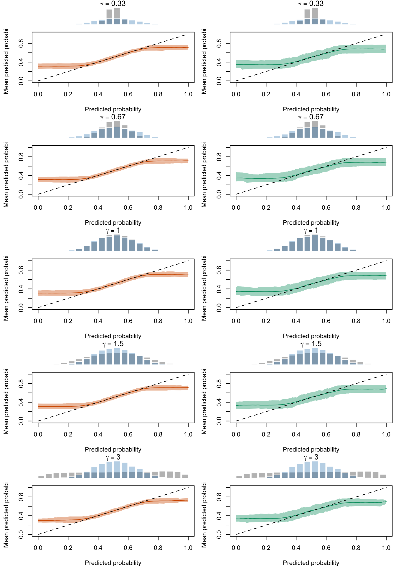
Contrary to the quantile-based calibration curve, we can make predictions on a segment from 0 to 1 using the fitted local regression.
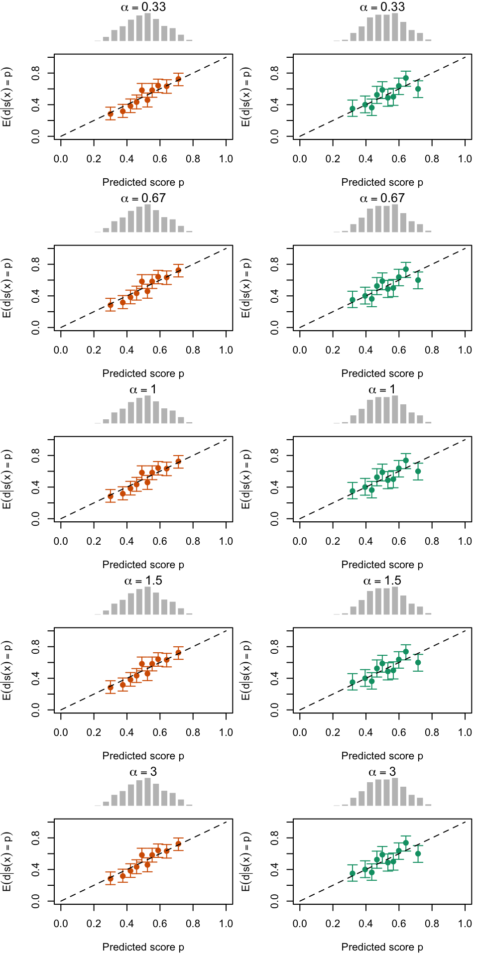
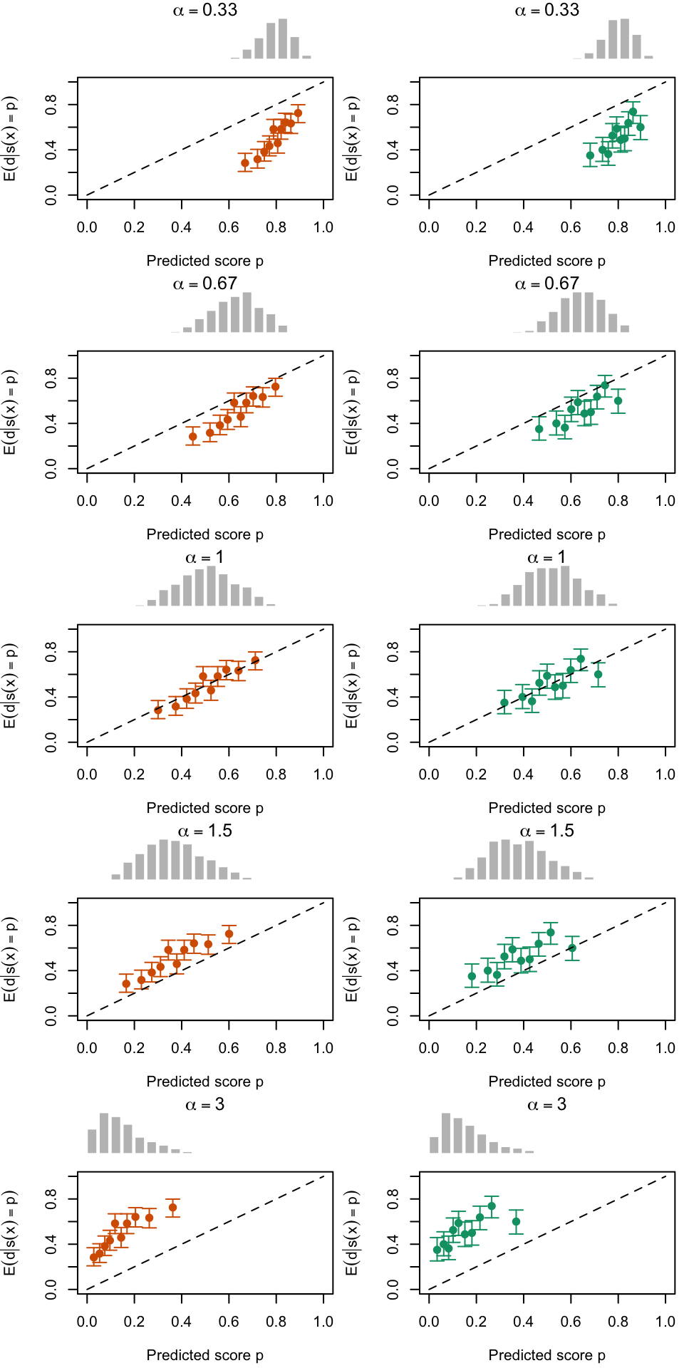
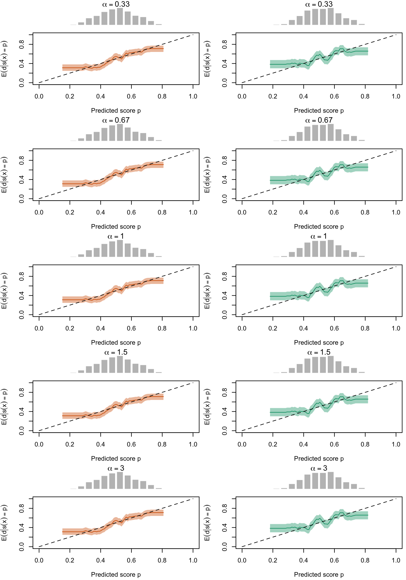
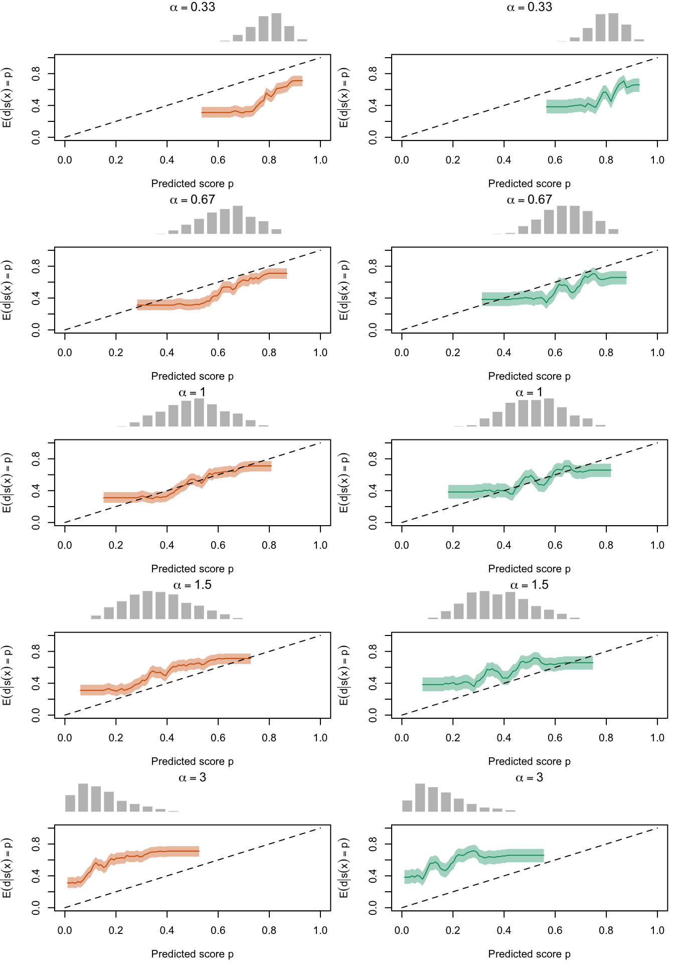
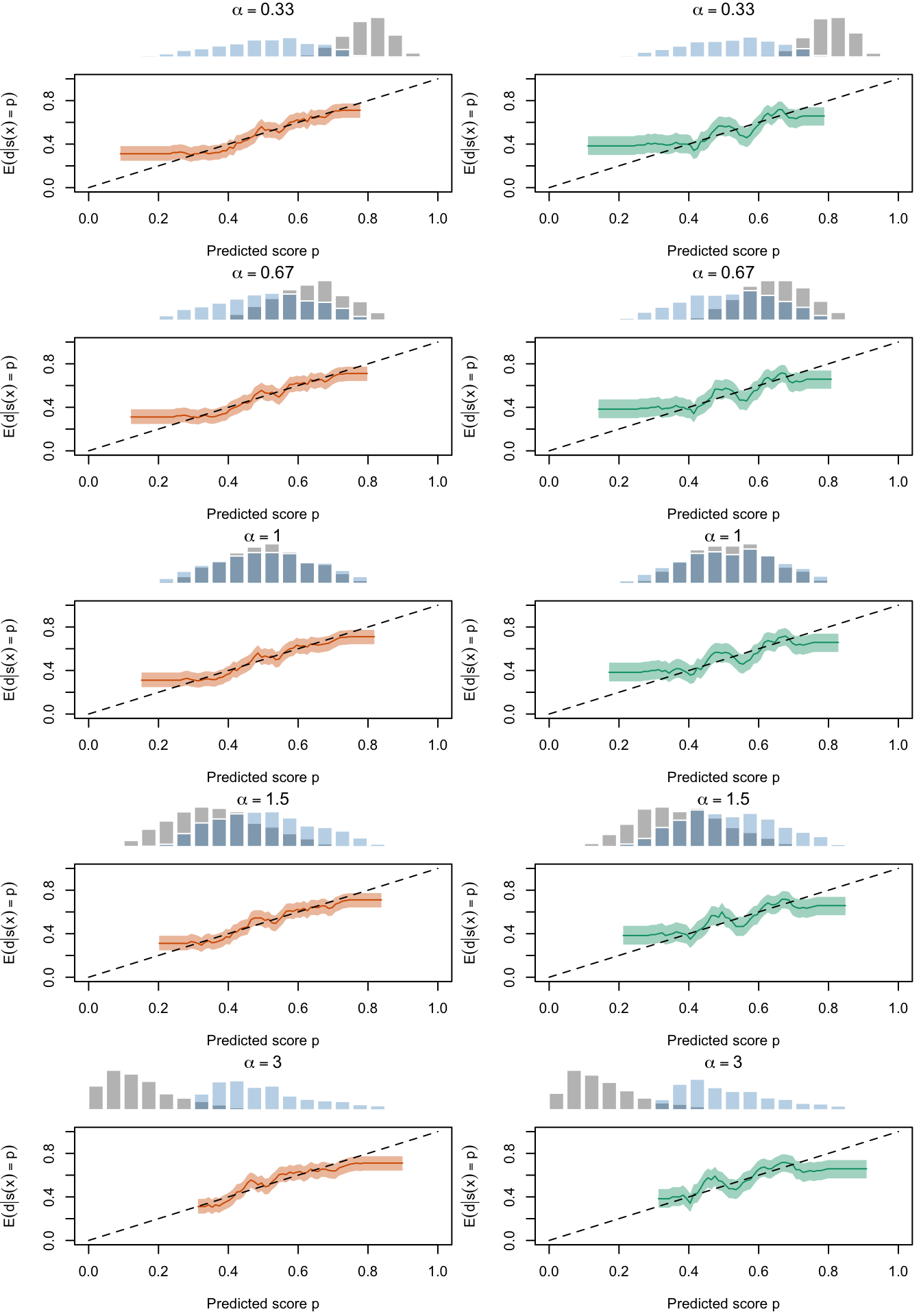
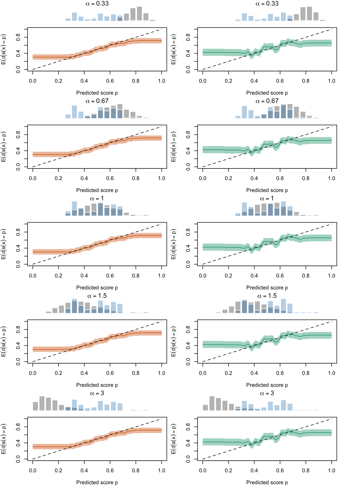
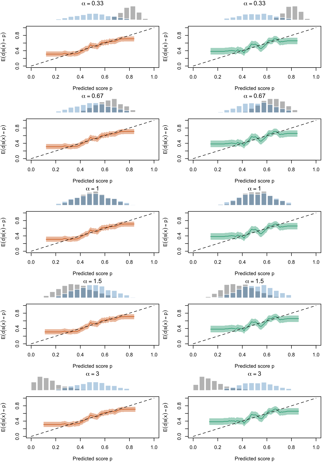
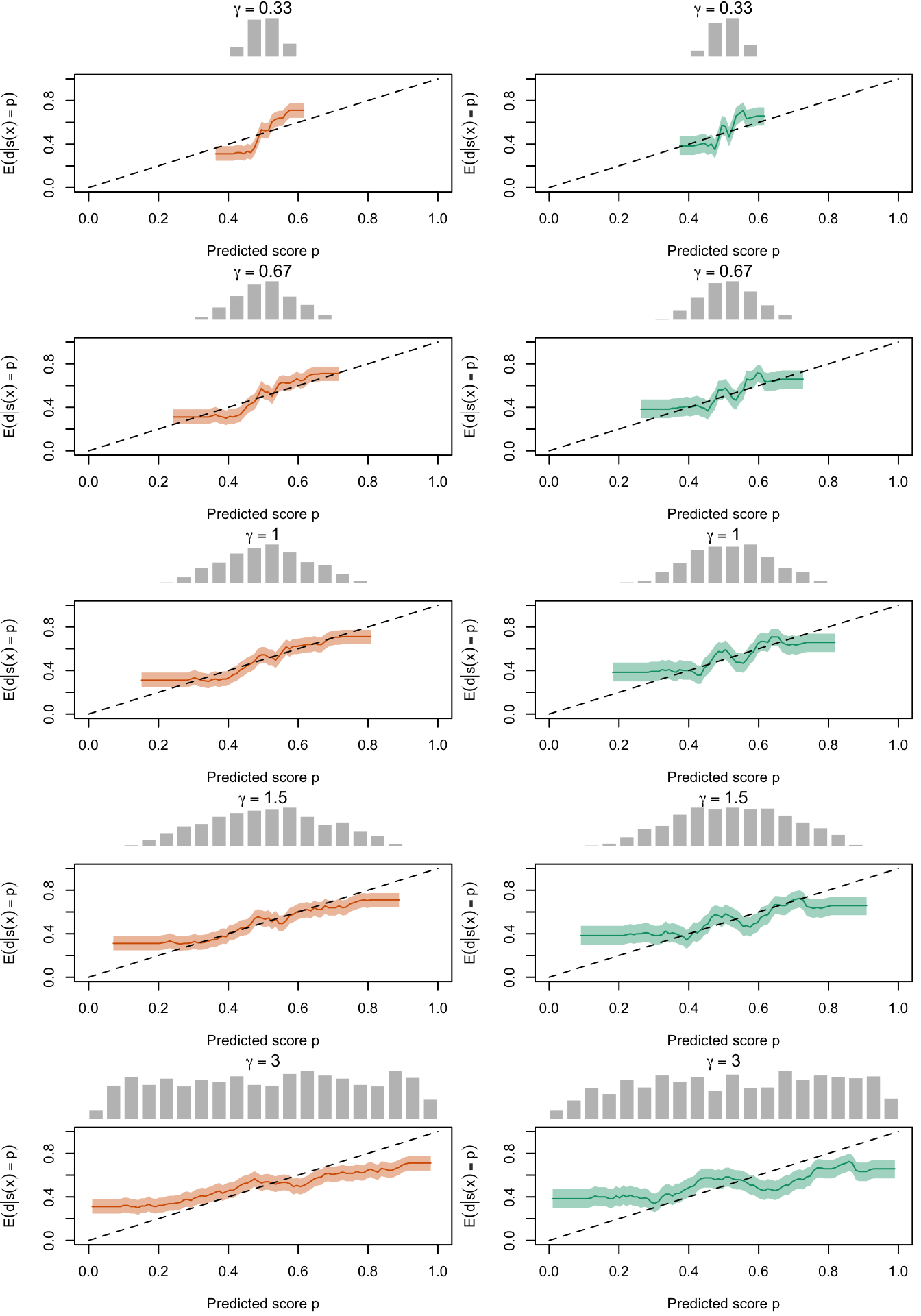
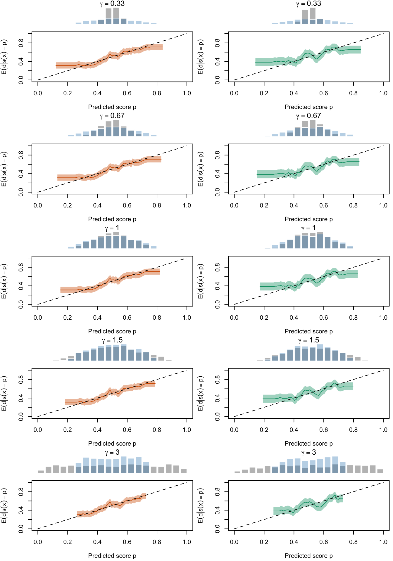
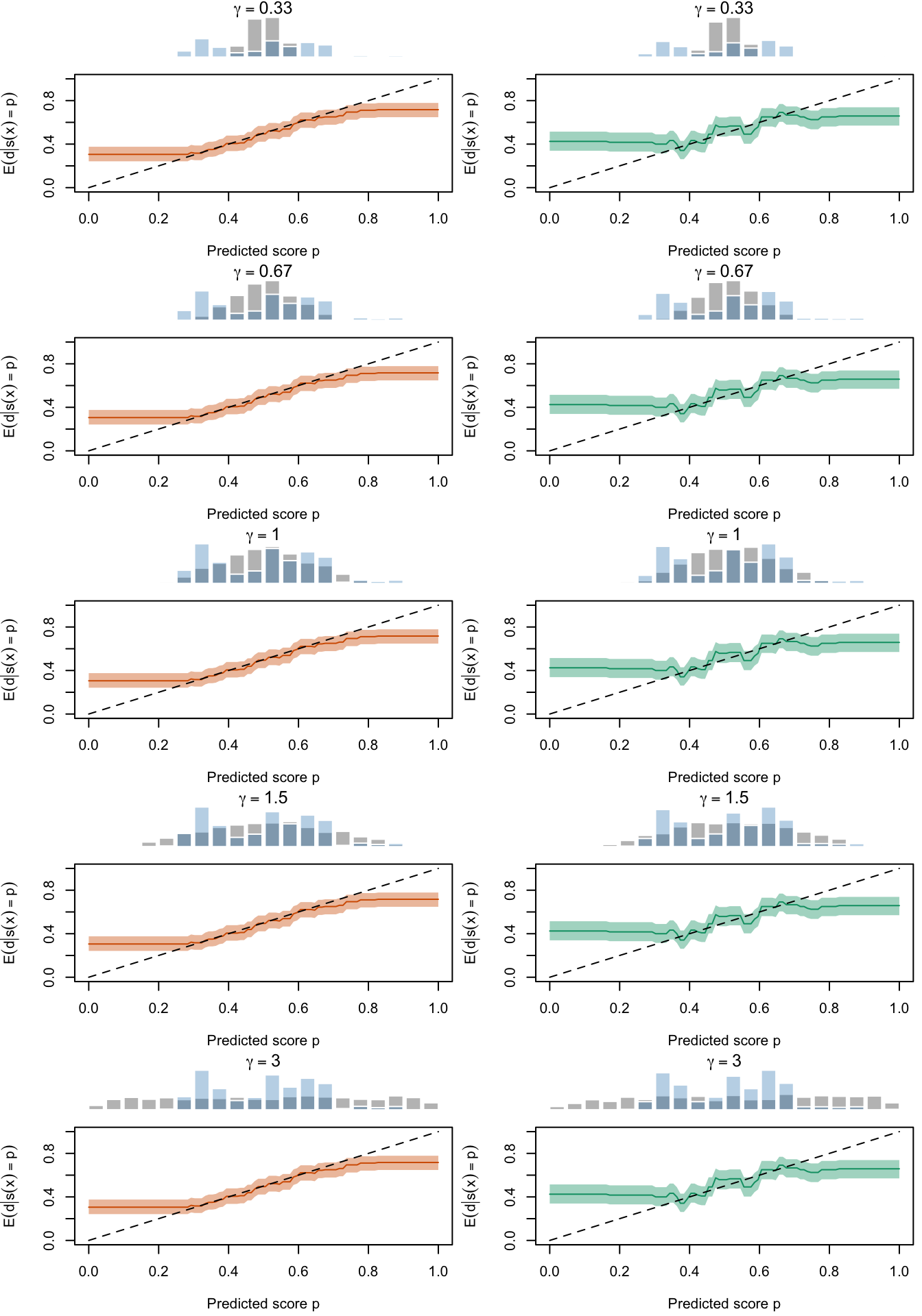
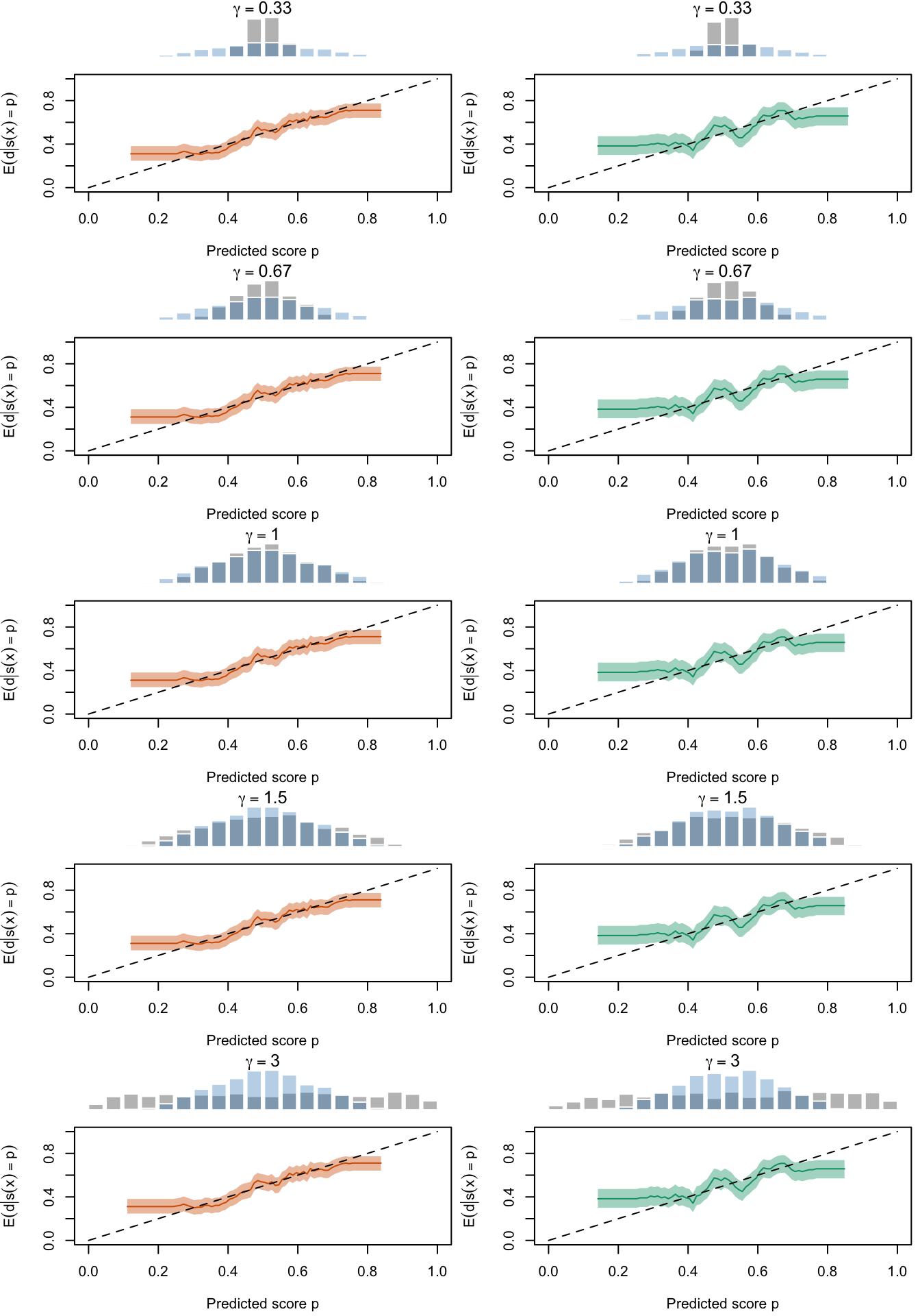
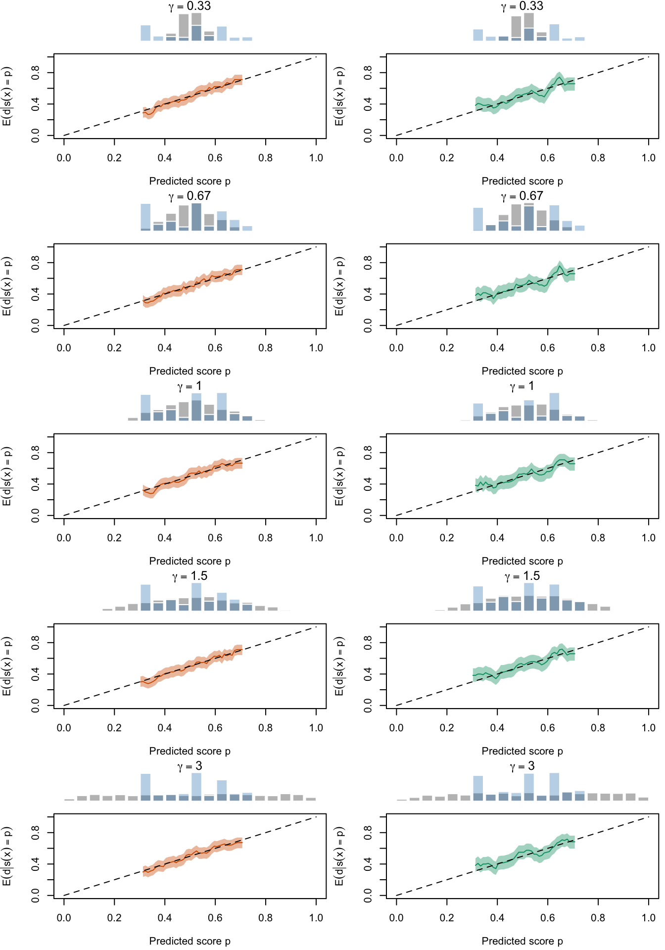
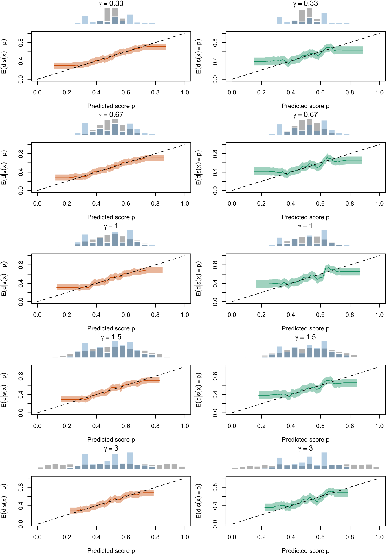
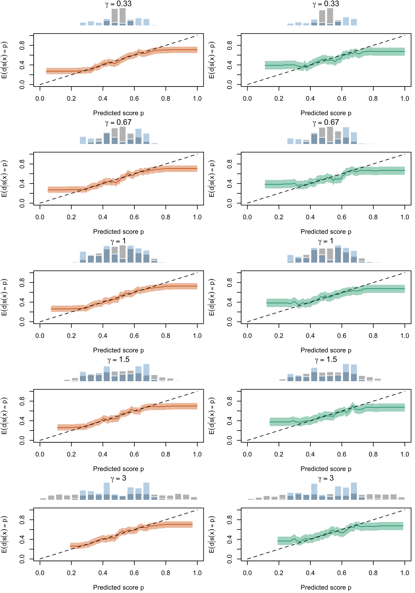
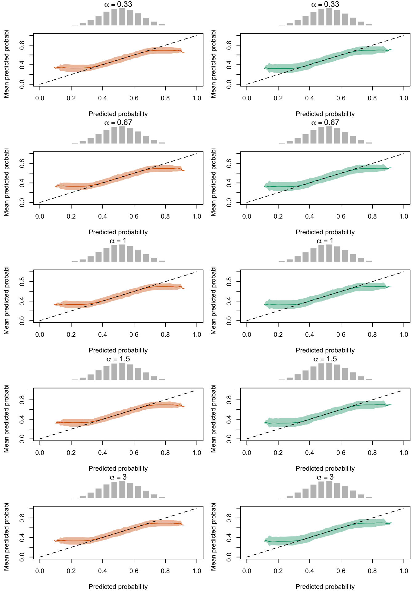
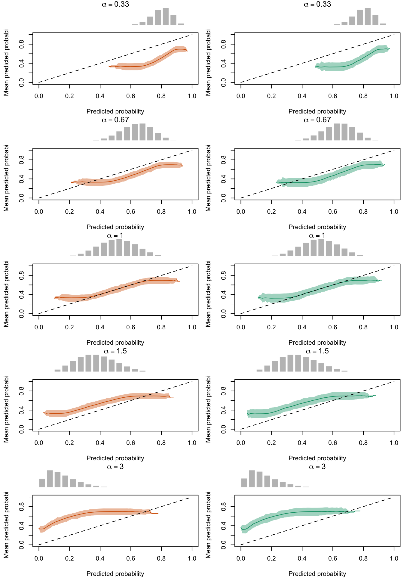
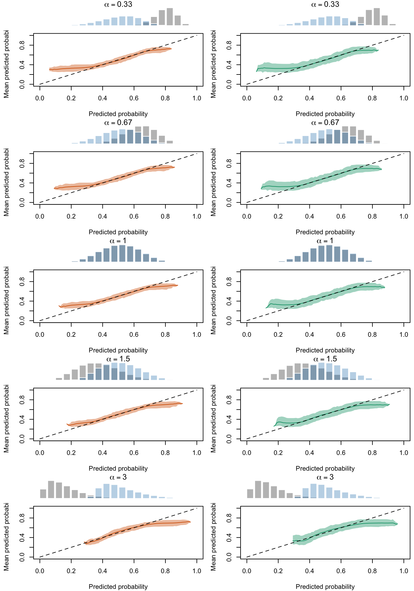
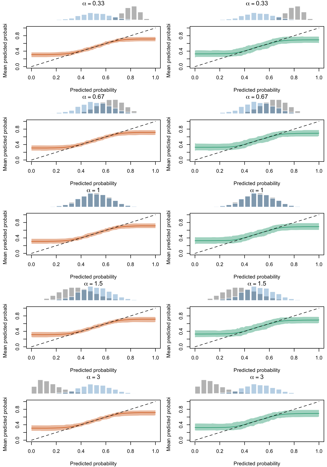
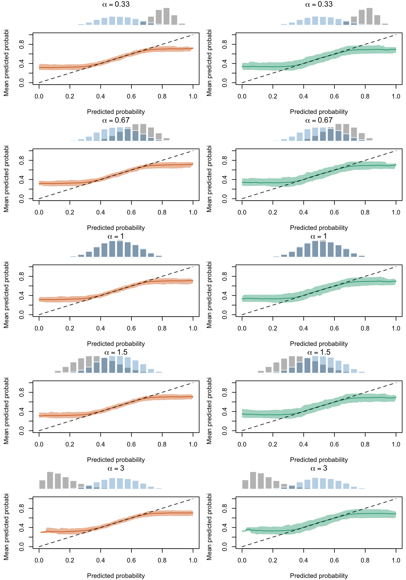
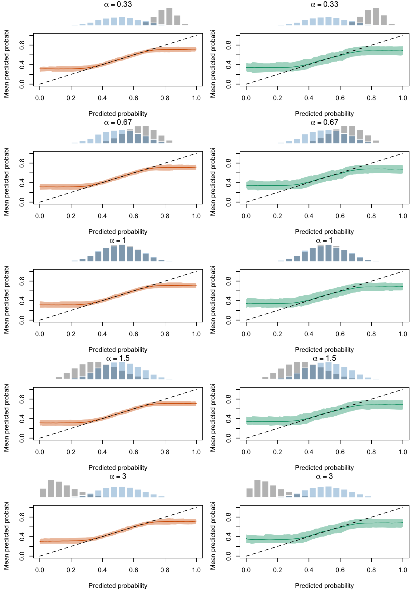
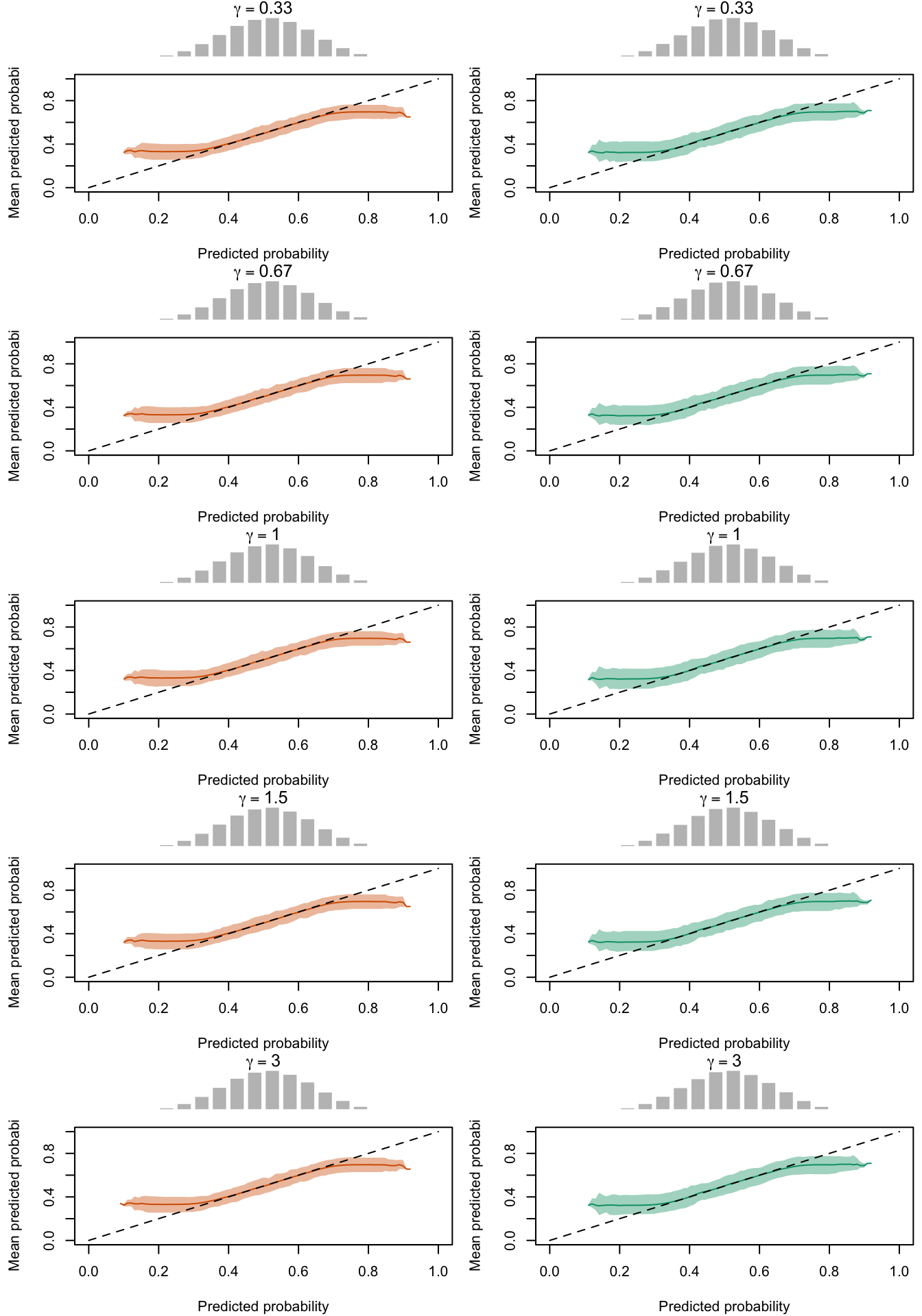
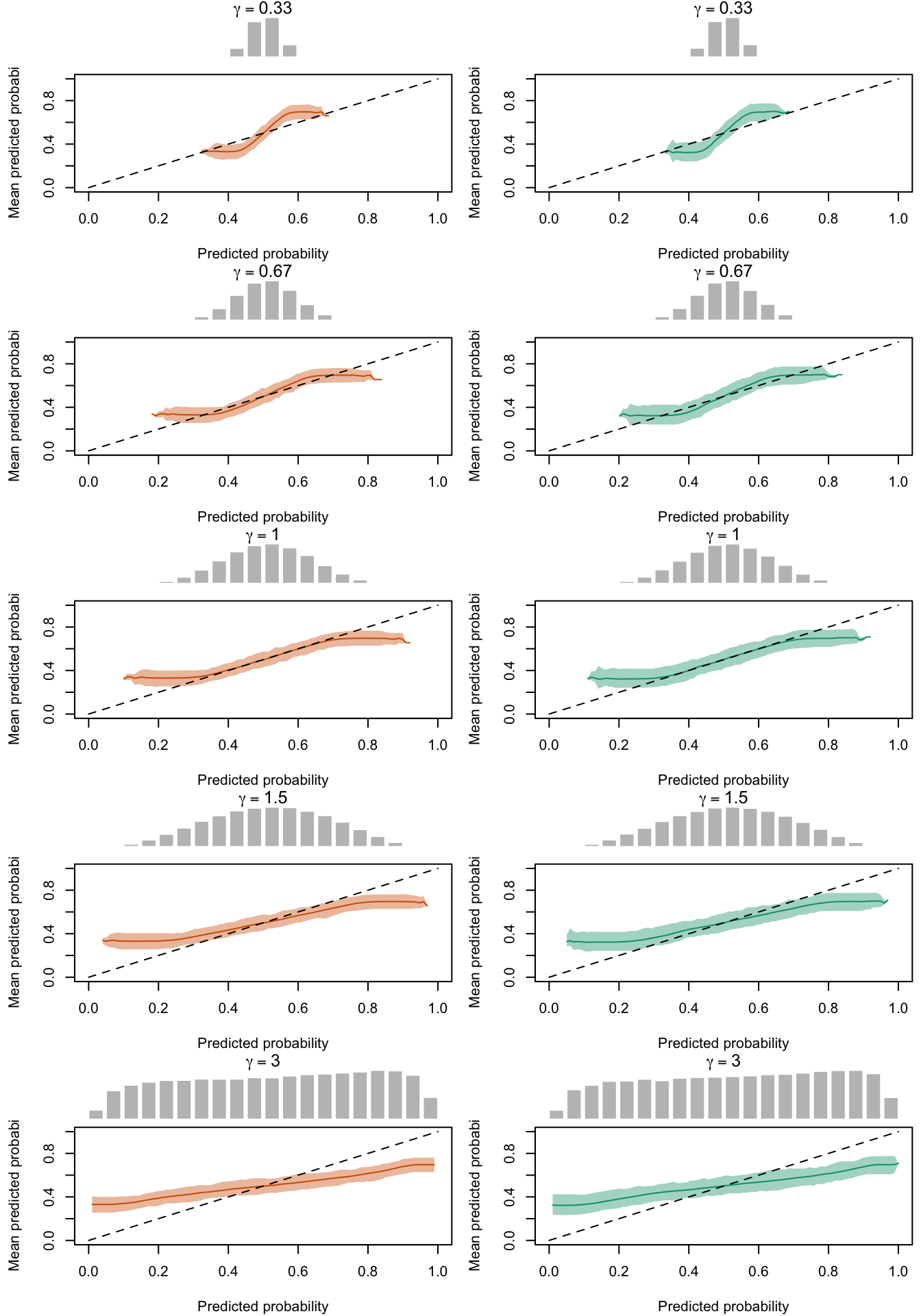
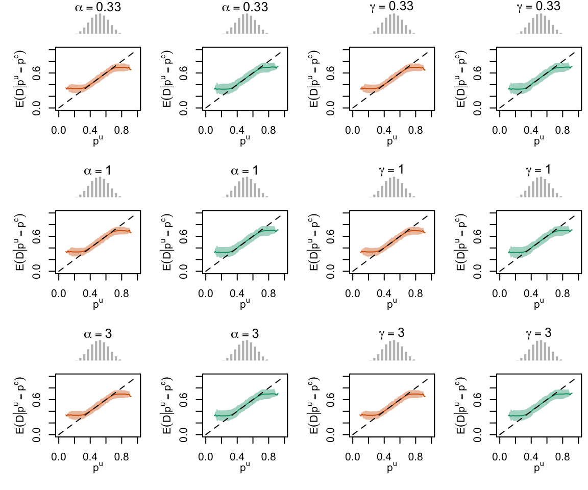
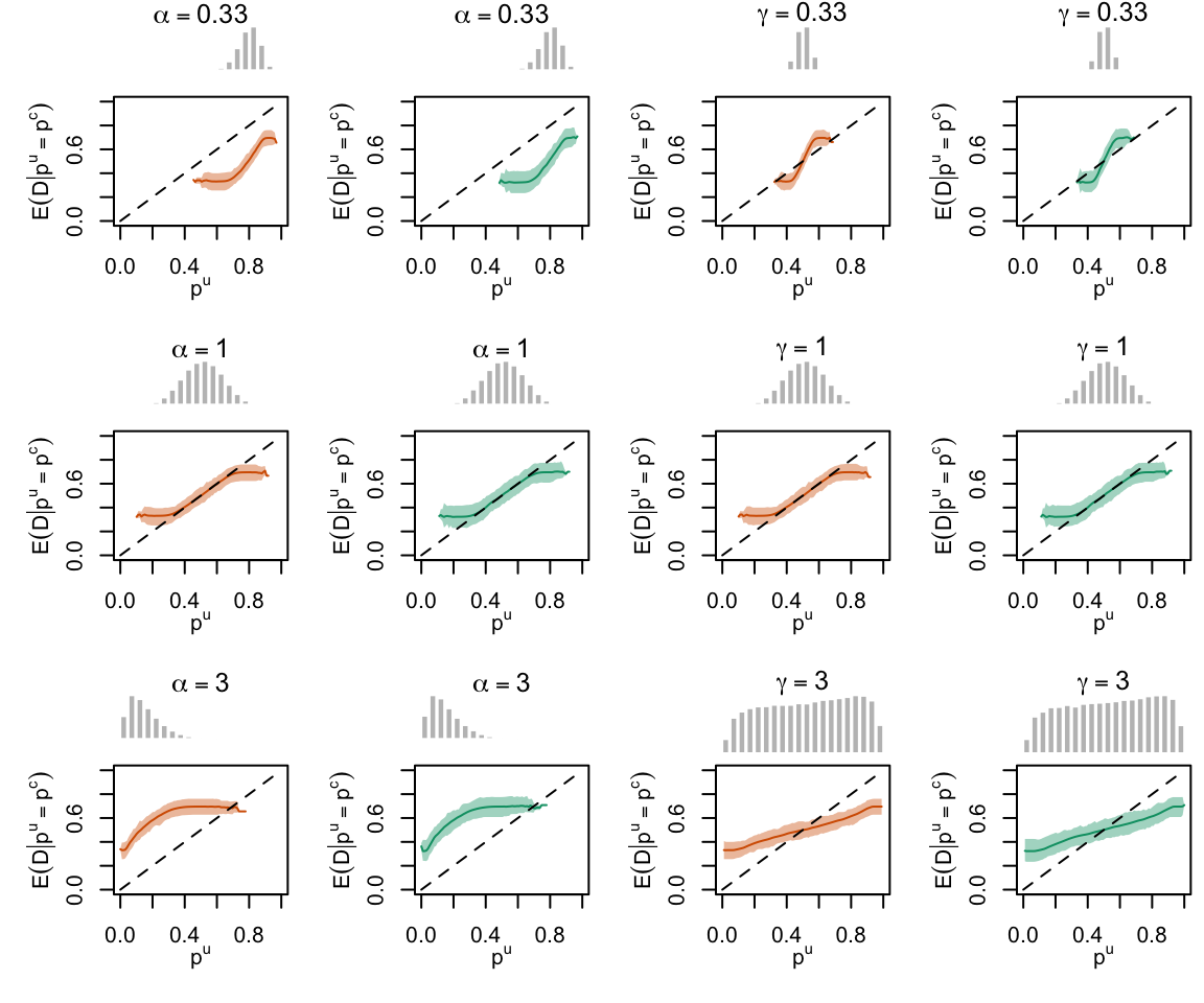
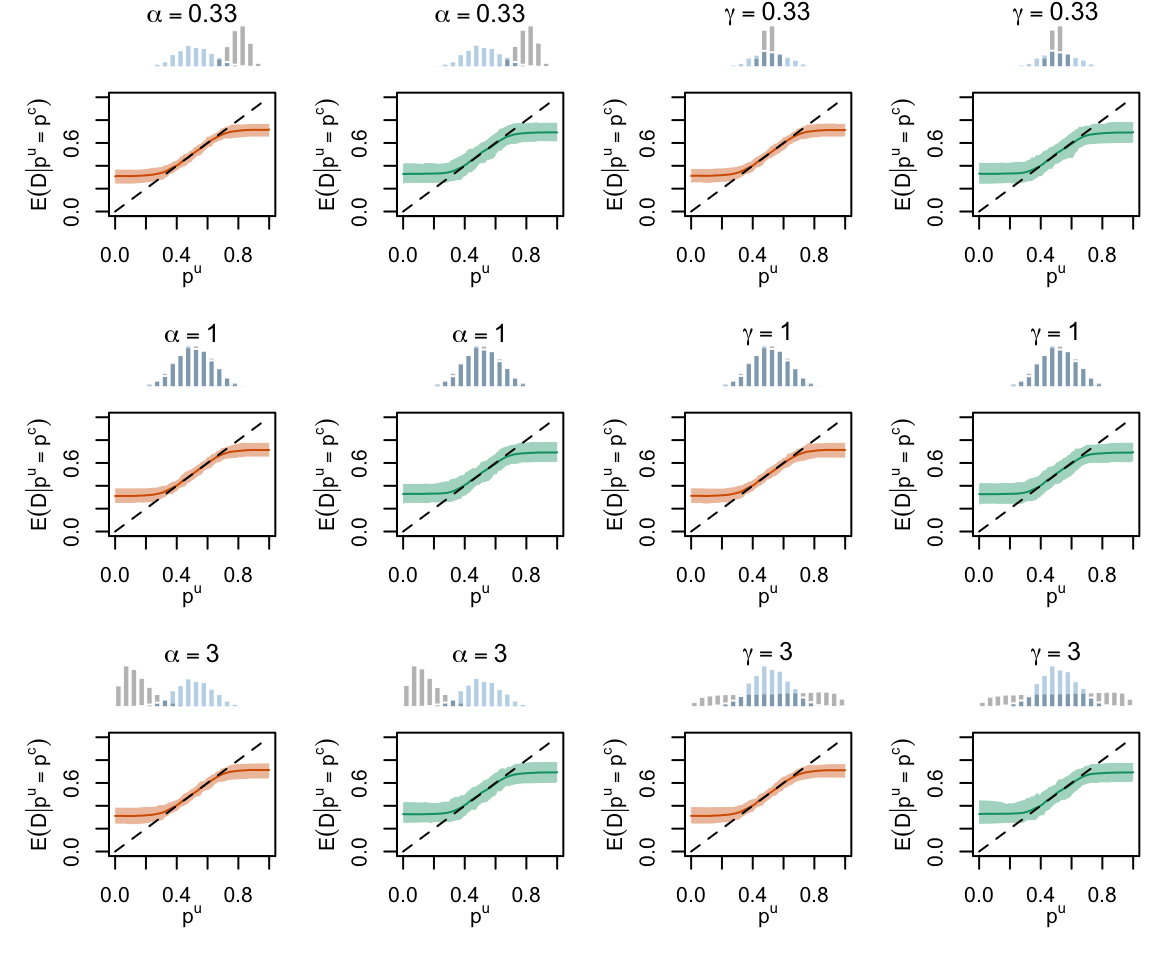
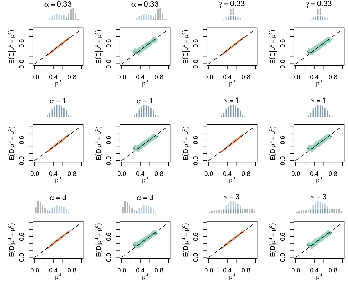
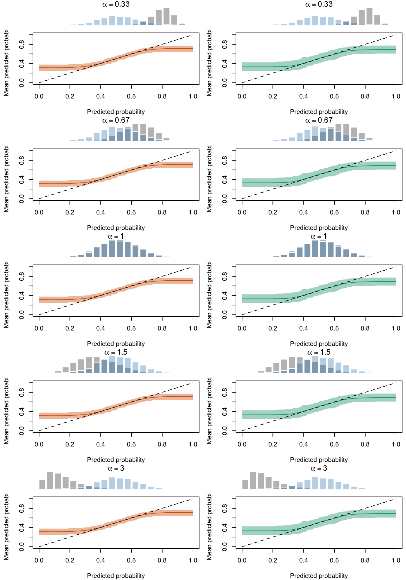
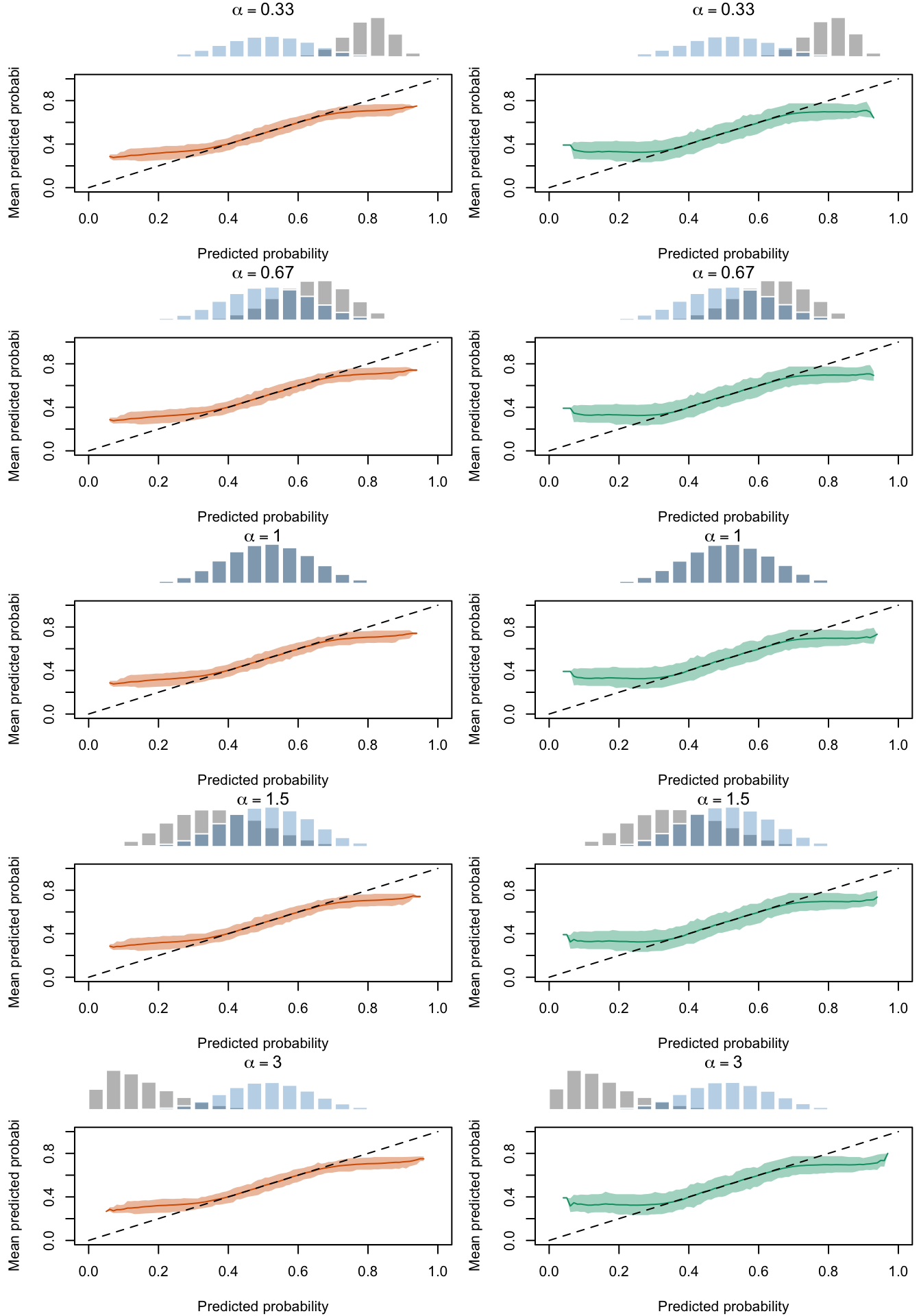
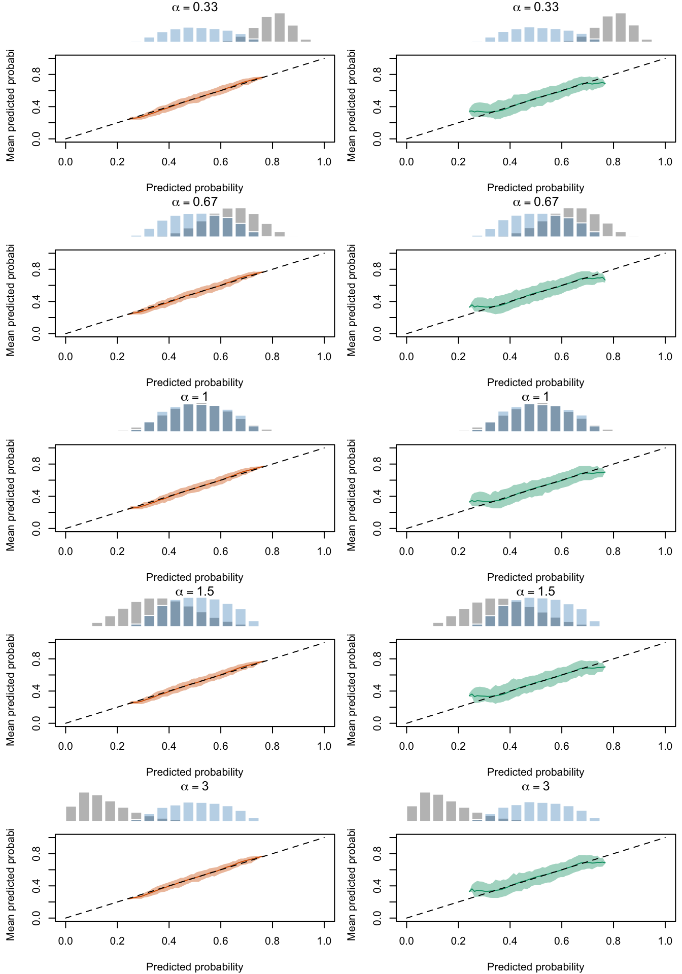
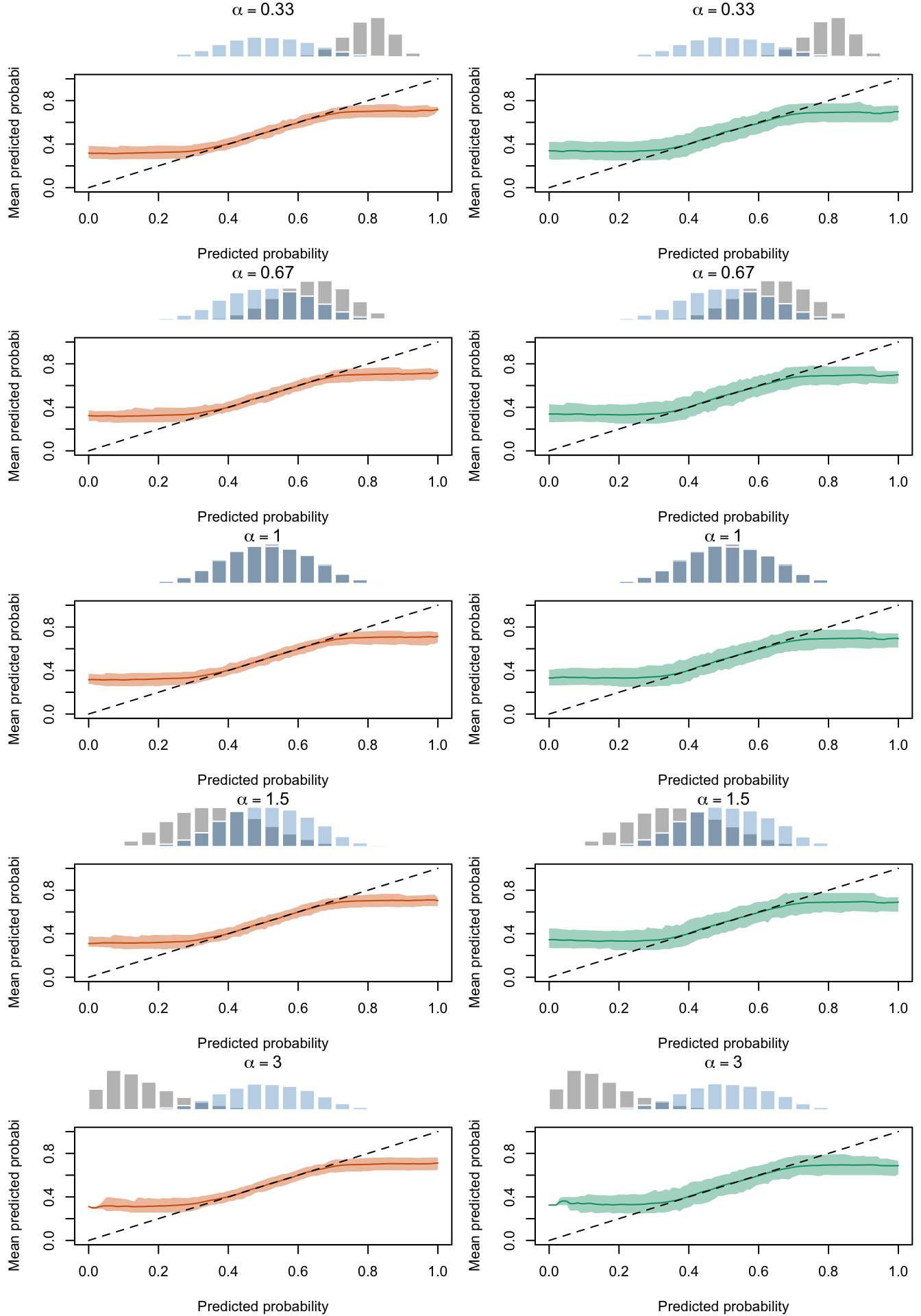
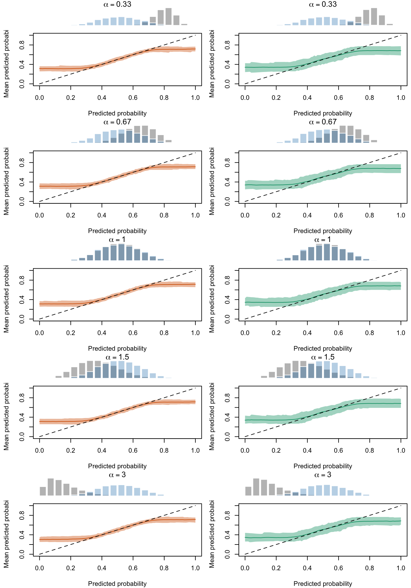
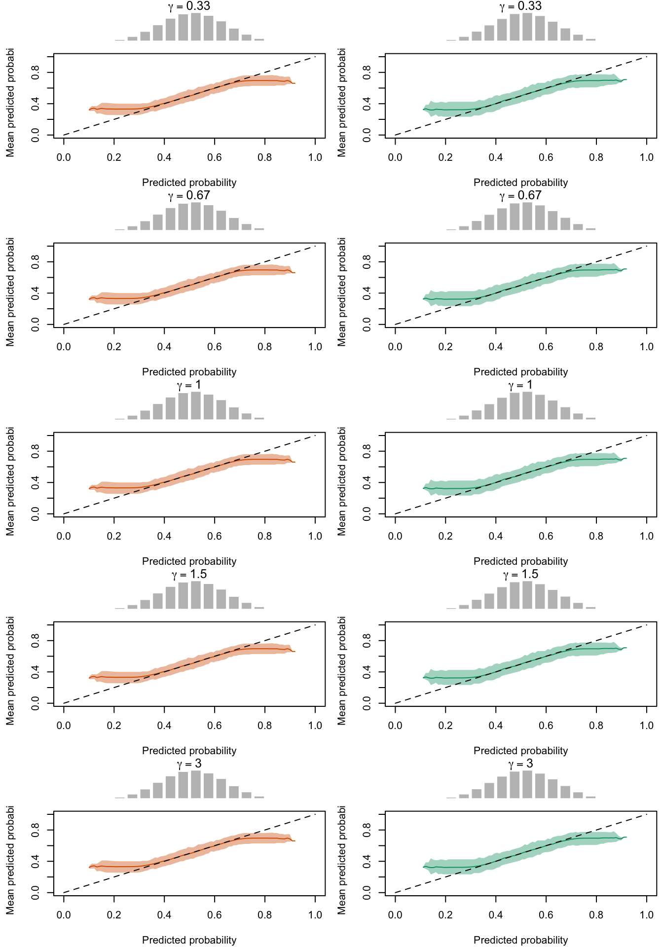
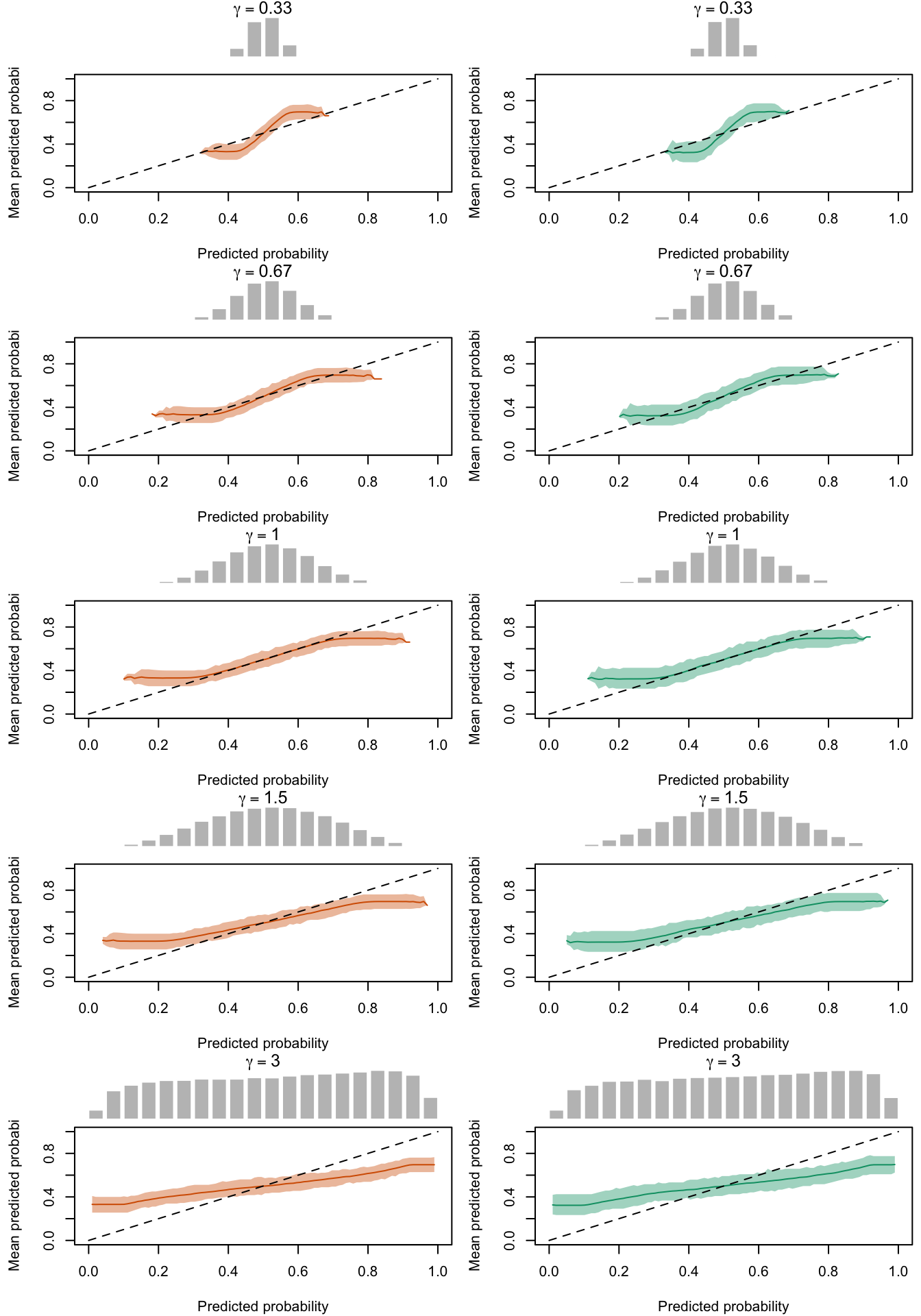
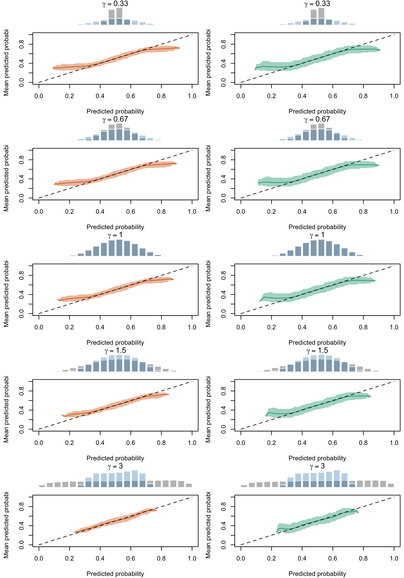
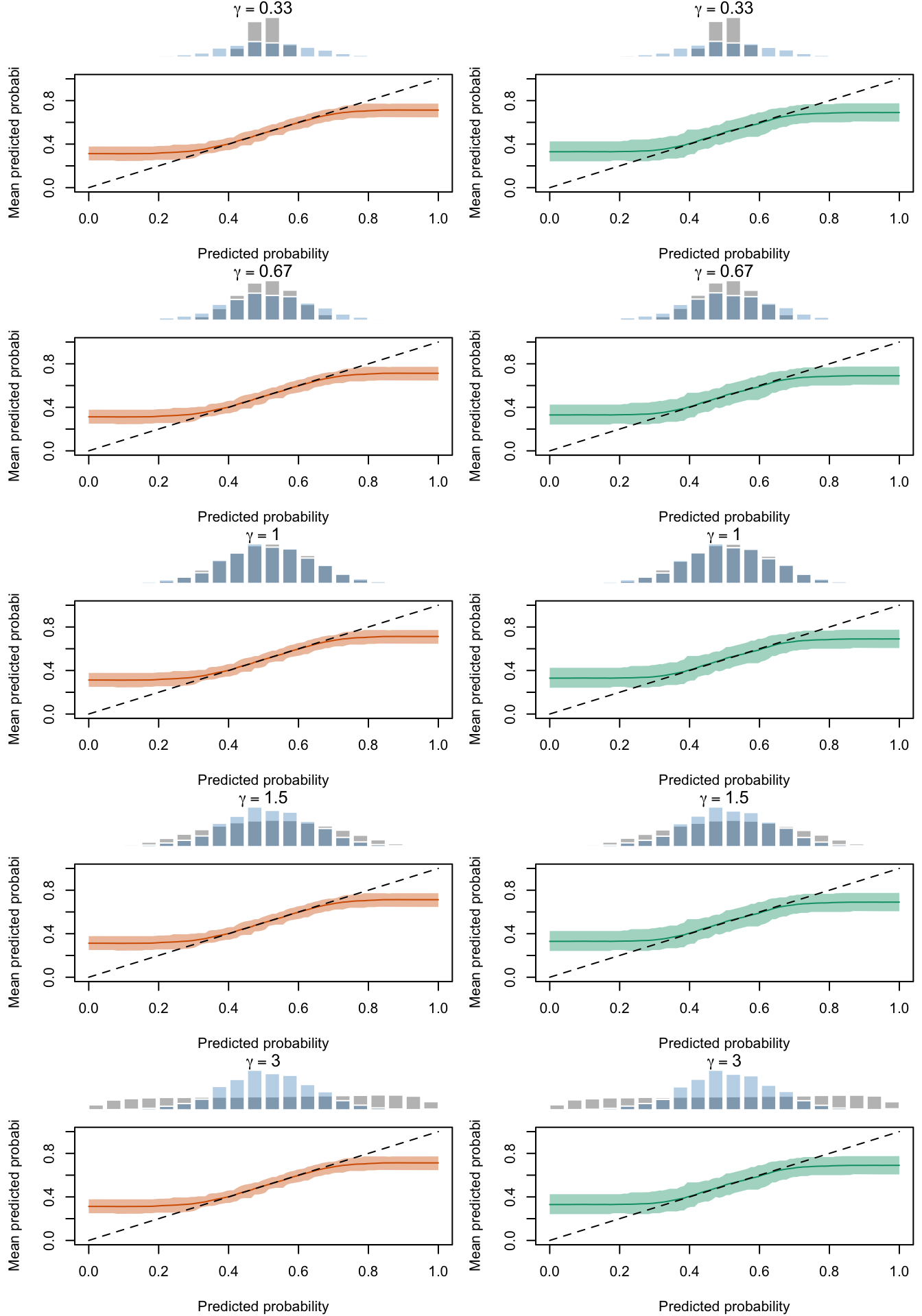
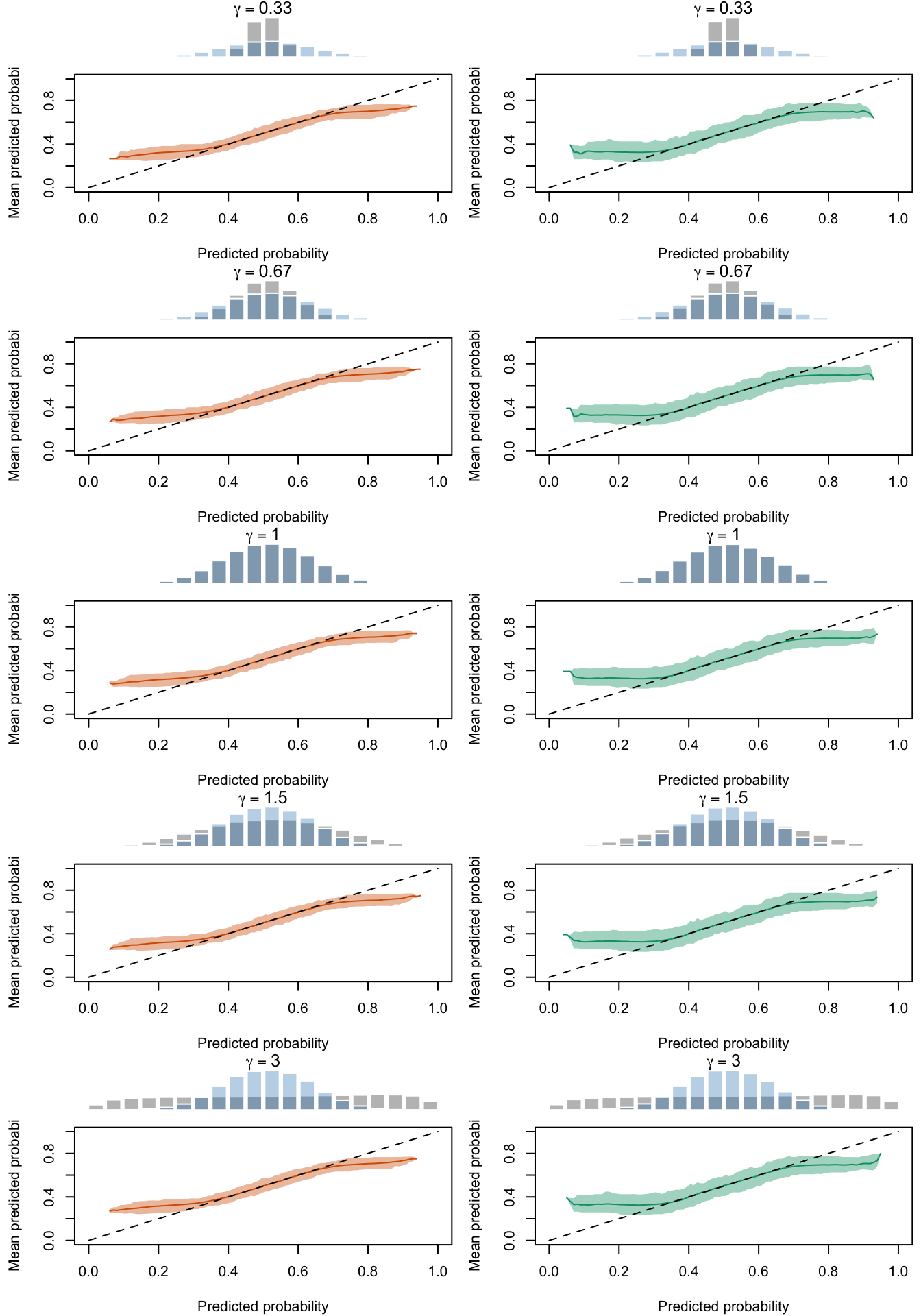
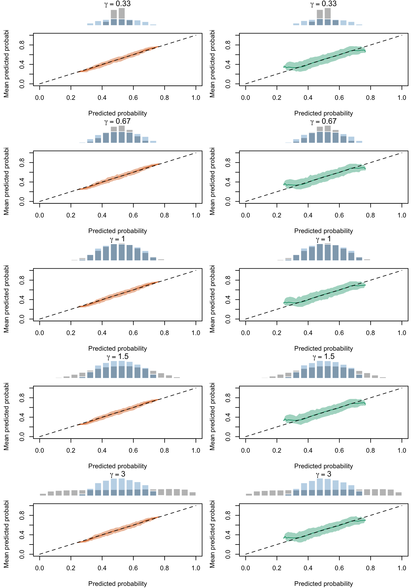
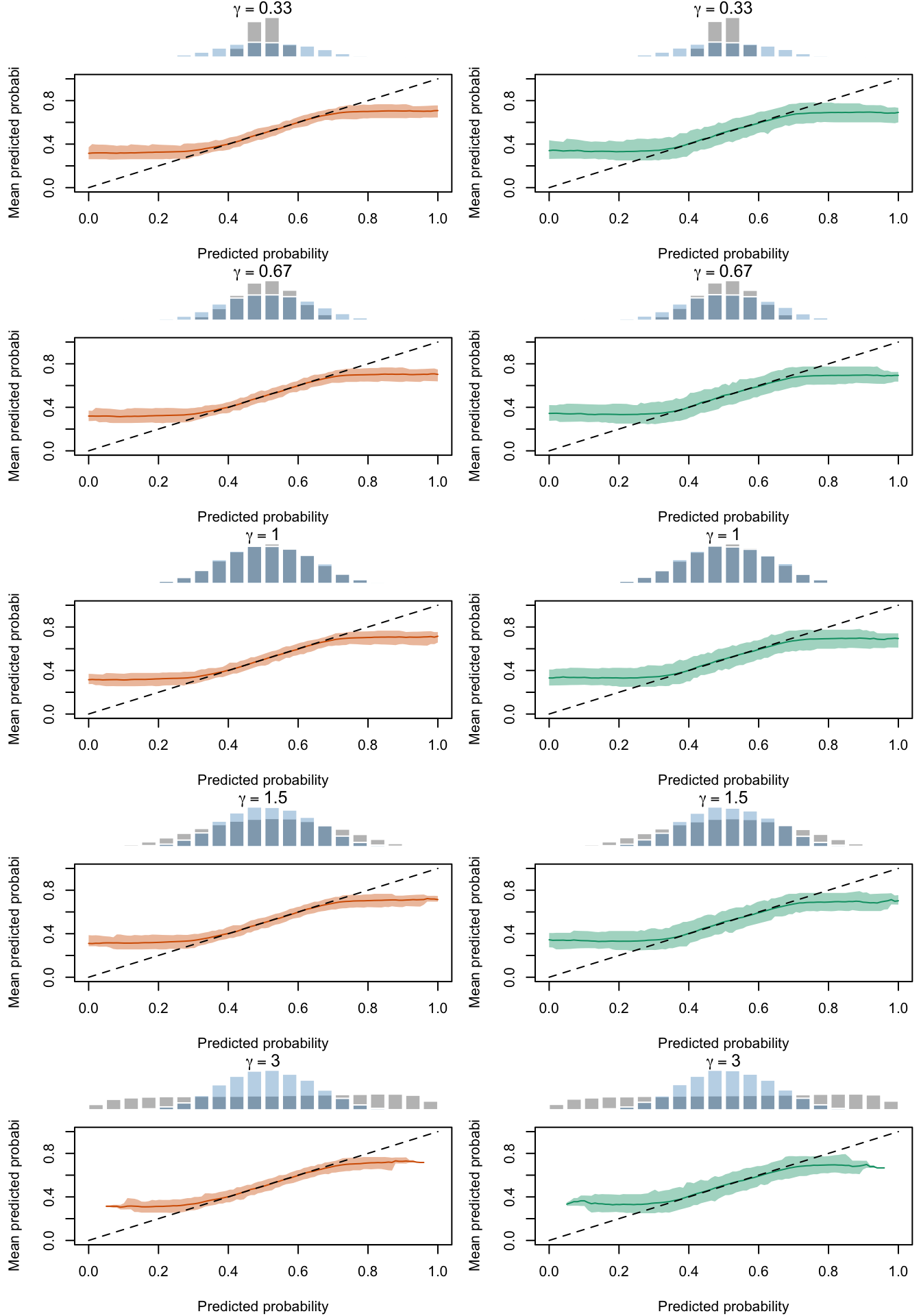
The figures below show a panel of graphs with the calibration curves obtained with the local regression method. Each tab shows the average curve obtained on the 200 replications for a type of recalibration used, as well as the 95% bootstrap confidence intervals. The first two tab (True Prob. and No Calibration) show the curves obtained using the true probabilities \(p\) and the uncalibrated probabilities \(p^u\), instead of the recalibrated probabilities \(p^c\). Each row of the panel in the Figures corresponds to a value for either \(\alpha\) or \(\gamma\) used to transform \(p\) to get \(p^u\). The left column shows the calibration curve obtained on the calibration set whereas the right column shows the calibration curve obtained on the test set. The average distribution (computed over the 200 simulations) of the uncalibrated scores and of the calibrated scores are shown in the histograms on top of each graph.
Calibration curves obtained with recalibrated scores. The curves are obtained with local regressions for the calibration set (left) and for the test set (right) for varying values of \(\alpha\) for 200 replication of the simulations. The histogram on top of each graph show the distribution of the uncalibrated scores, and that of the calibrated scores
Calibration curves obtained with recalibrated scores. The curves are obtained with local regressions for the calibration set (left) and for the test set (right) for varying values of \(\alpha\) for 200 replication of the simulations. The histogram on top of each graph show the distribution of the uncalibrated scores, and that of the calibrated scores
Calibration curves obtained with recalibrated scores. The curves are obtained with local regressions for the calibration set (left) and for the test set (right) for varying values of \(\alpha\) for 200 replication of the simulations. The histogram on top of each graph show the distribution of the uncalibrated scores, and that of the calibrated scores
Calibration curves obtained with recalibrated scores. The curves are obtained with local regressions for the calibration set (left) and for the test set (right) for varying values of \(\alpha\) for 200 replication of the simulations. The histogram on top of each graph show the distribution of the uncalibrated scores, and that of the calibrated scores
Calibration curves obtained with recalibrated scores. The curves are obtained with local regressions for the calibration set (left) and for the test set (right) for varying values of \(\alpha\) for 200 replication of the simulations. The histogram on top of each graph show the distribution of the uncalibrated scores, and that of the calibrated scores
Calibration curves obtained with recalibrated scores. The curves are obtained with local regressions for the calibration set (left) and for the test set (right) for varying values of \(\alpha\) for 200 replication of the simulations. The histogram on top of each graph show the distribution of the uncalibrated scores, and that of the calibrated scores
Calibration curves obtained with recalibrated scores. The curves are obtained with local regressions for the calibration set (left) and for the test set (right) for varying values of \(\alpha\) for 200 replication of the simulations. The histogram on top of each graph show the distribution of the uncalibrated scores, and that of the calibrated scores
Calibration curves obtained with recalibrated scores. The curves are obtained with local regressions for the calibration set (left) and for the test set (right) for varying values of \(\alpha\) for 200 replication of the simulations. The histogram on top of each graph show the distribution of the uncalibrated scores, and that of the calibrated scores
Calibration curves obtained with recalibrated scores. The curves are obtained with local regressions for the calibration set (left) and for the test set (right) for varying values of \(\gamma\) for 200 replication of the simulations. The histogram on top of each graph show the distribution of the uncalibrated scores, and that of the calibrated scores
Calibration curves obtained with recalibrated scores. The curves are obtained with local regressions for the calibration set (left) and for the test set (right) for varying values of \(\gamma\) for 200 replication of the simulations. The histogram on top of each graph show the distribution of the uncalibrated scores, and that of the calibrated scores
Calibration curves obtained with recalibrated scores. The curves are obtained with local regressions for the calibration set (left) and for the test set (right) for varying values of \(\gamma\) for 200 replication of the simulations. The histogram on top of each graph show the distribution of the uncalibrated scores, and that of the calibrated scores
Calibration curves obtained with recalibrated scores. The curves are obtained with local regressions for the calibration set (left) and for the test set (right) for varying values of \(\gamma\) for 200 replication of the simulations. The histogram on top of each graph show the distribution of the uncalibrated scores, and that of the calibrated scores
Calibration curves obtained with recalibrated scores. The curves are obtained with local regressions for the calibration set (left) and for the test set (right) for varying values of \(\gamma\) for 200 replication of the simulations. The histogram on top of each graph show the distribution of the uncalibrated scores, and that of the calibrated scores
Calibration curves obtained with recalibrated scores. The curves are obtained with local regressions for the calibration set (left) and for the test set (right) for varying values of \(\gamma\) for 200 replication of the simulations. The histogram on top of each graph show the distribution of the uncalibrated scores, and that of the calibrated scores
Calibration curves obtained with recalibrated scores. The curves are obtained with local regressions for the calibration set (left) and for the test set (right) for varying values of \(\gamma\) for 200 replication of the simulations. The histogram on top of each graph show the distribution of the uncalibrated scores, and that of the calibrated scores
Calibration curves obtained with recalibrated scores. The curves are obtained with local regressions for the calibration set (left) and for the test set (right) for varying values of \(\gamma\) for 200 replication of the simulations. The histogram on top of each graph show the distribution of the uncalibrated scores, and that of the calibrated scores
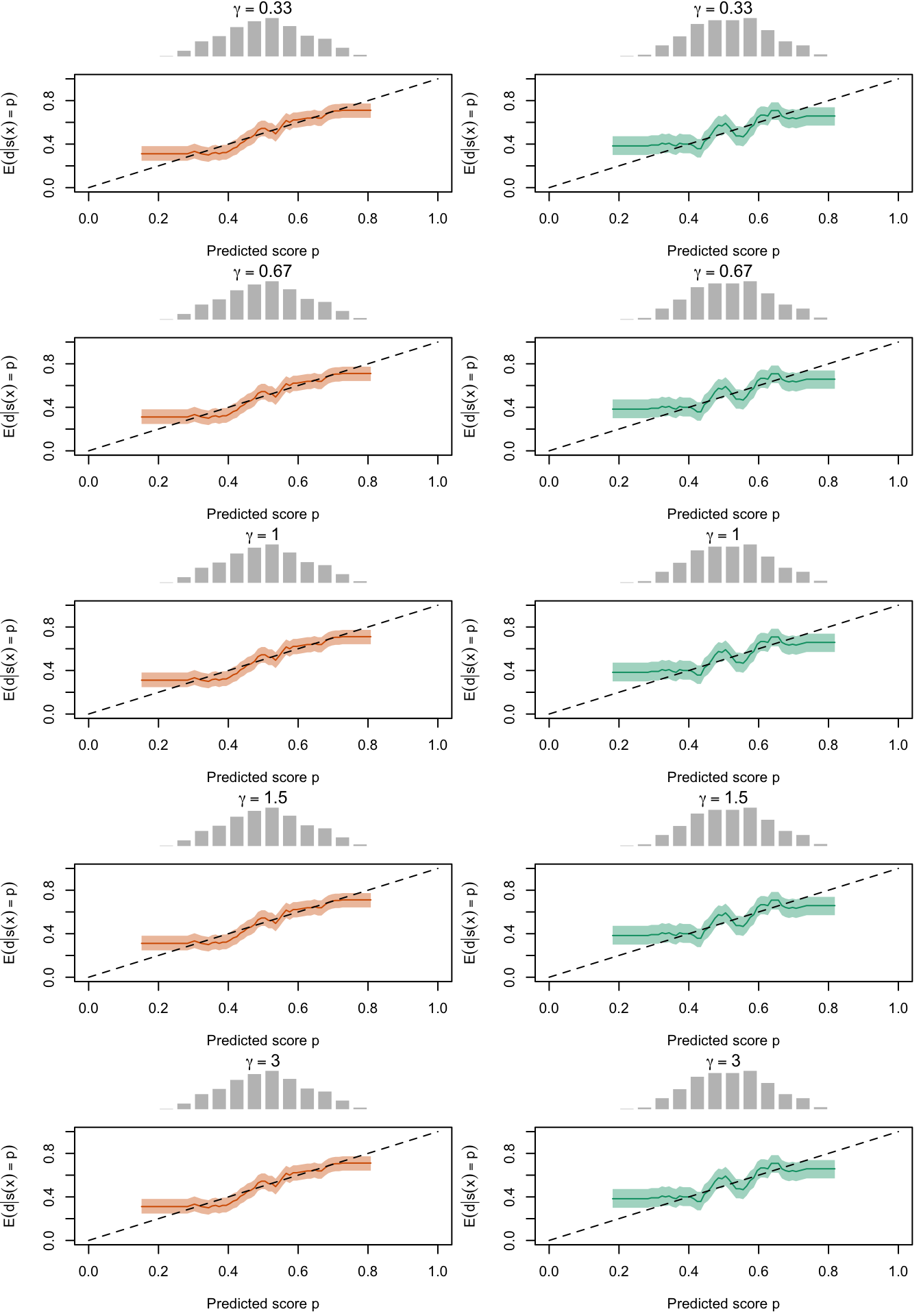
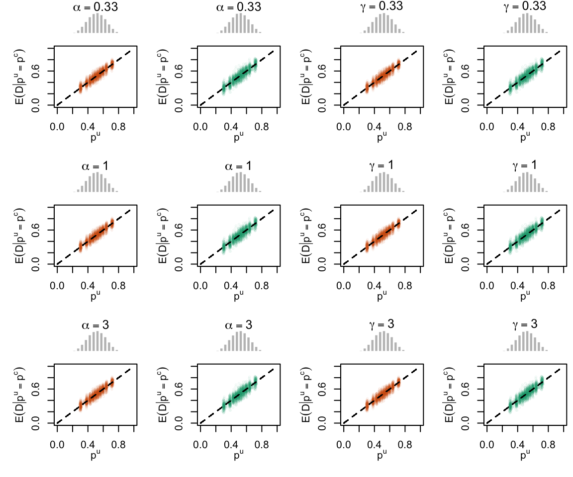
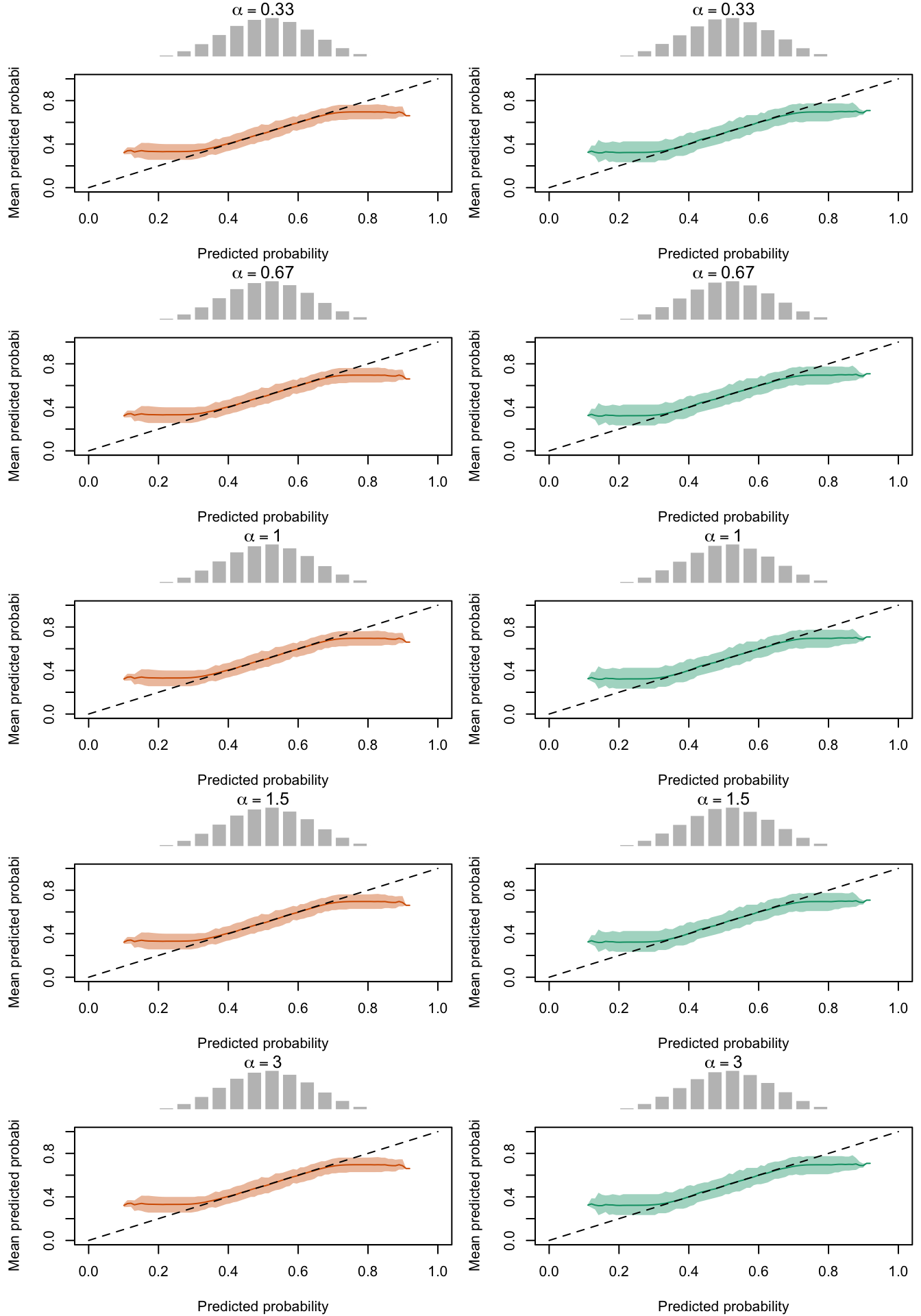
Figure 2.27: Calibration Curves Calculated with True Probabilities as the Scores. The curves are obtained with quantile binning, for the calibration set (orange) and for the test set (green) for varying values of \(\alpha\) and \(\gamma\). The curves are the average values obtained on 200 replications of the simulations, the bands correspond to 95% bootstrap interval. The histogram on top of each graph show the distribution of the true probabilities
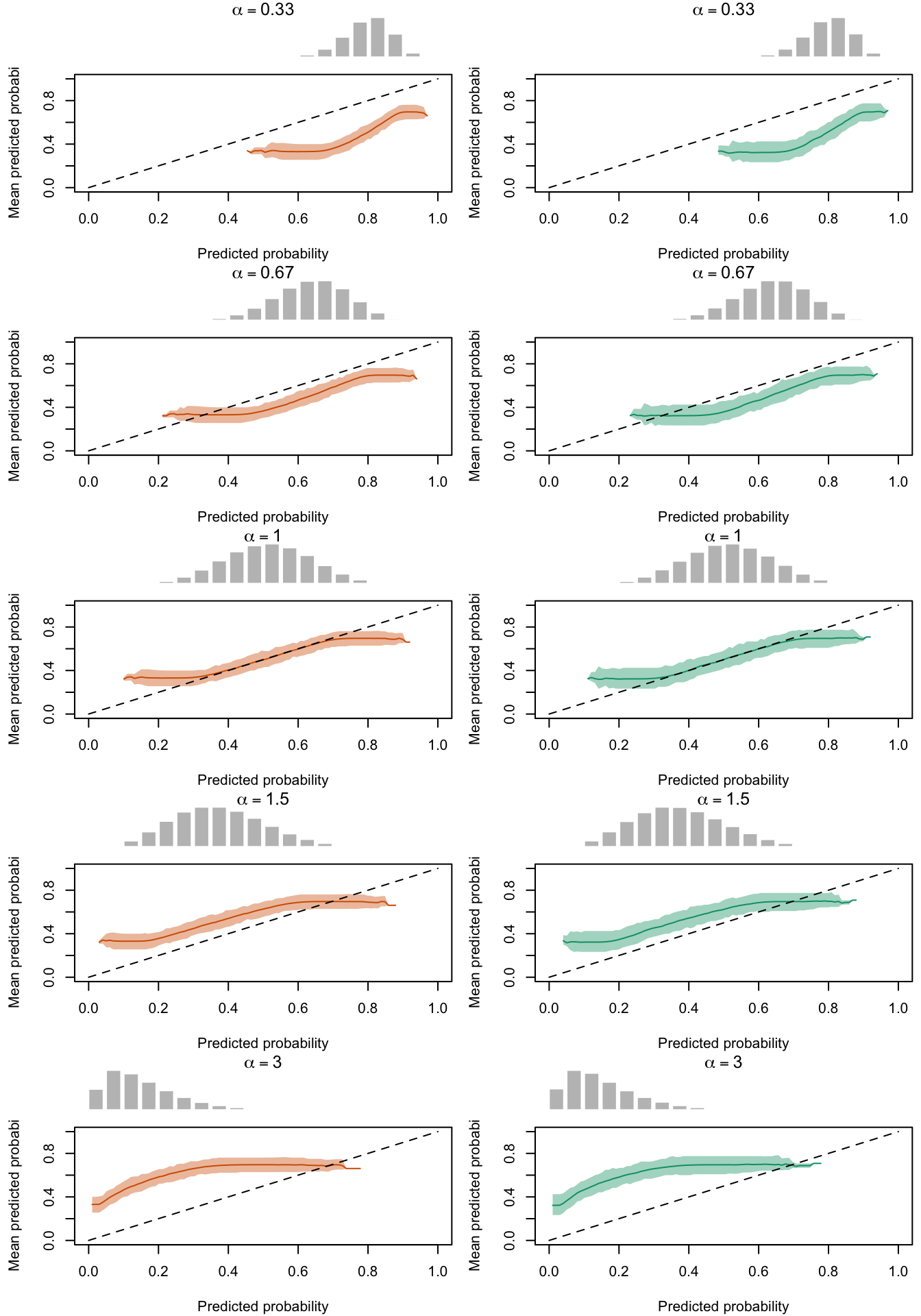
Figure 2.28: Calibration Curves Calculated with Uncalibrated Scores. The curves are obtained with quantile binning, for the calibration set (orange) and for the test set (green) for varying values of \(\alpha\) and \(\gamma\). The curves are the average values obtained on 200 replications of the simulations, the bands correspond to 95% bootstrap interval. The histogram on top of each graph show the distribution of the true probabilities
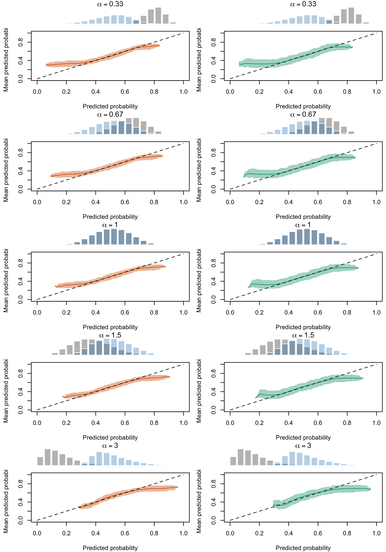
Figure 2.29: Calibration Curves Calculated with Scores Recalibrated Using Platt Scaling. The curves are obtained with quantile binning, for the calibration set (orange) and for the test set (green) for varying values of \(\alpha\) and \(\gamma\). The curves are the average values obtained on 200 replications of the simulations, the bands correspond to 95% bootstrap interval. The histogram on top of each graph show the distribution of the uncalibrated scores, and that of the calibrated scores
Figure 2.30: Calibration Curves Calculated with Scores Recalibrated Using Isotonic Regression. The curves are obtained with quantile binning, for the calibration set (orange) and for the test set (green) for varying values of \(\alpha\) and \(\gamma\). The curves are the average values obtained on 200 replications of the simulations, the bands correspond to 95% bootstrap interval. The histogram on top of each graph show the distribution of the uncalibrated scores, and that of the calibrated scores
Figure 2.31: Calibration Curves Calculated with Scores Recalibrated Using Beta Calibration. The curves are obtained with quantile binning, for the calibration set (orange) and for the test set (green) for varying values of \(\alpha\) and \(\gamma\). The curves are the average values obtained on 200 replications of the simulations, the bands correspond to 95% bootstrap interval. The histogram on top of each graph show the distribution of the uncalibrated scores, and that of the calibrated scores
Figure 2.32: Calibration Curves Calculated with Scores Recalibrated Using Local Regression (with degree 0). The curves are obtained with quantile binning, for the calibration set (orange) and for the test set (green) for varying values of \(\alpha\) and \(\gamma\). The curves are the average values obtained on 200 replications of the simulations, the bands correspond to 95% bootstrap interval. The histogram on top of each graph show the distribution of the uncalibrated scores, and that of the calibrated scores
Figure 2.33: Calibration Curves Calculated with Scores Recalibrated Using Local Regression (with degree 1). The curves are obtained with quantile binning, for the calibration set (orange) and for the test set (green) for varying values of \(\alpha\) and \(\gamma\). The curves are the average values obtained on 200 replications of the simulations, the bands correspond to 95% bootstrap interval. The histogram on top of each graph show the distribution of the uncalibrated scores, and that of the calibrated scores
Figure 2.34: Calibration Curves Calculated with Scores Recalibrated Using Local Regression (with degree 2). The curves are obtained with quantile binning, for the calibration set (orange) and for the test set (green) for varying values of \(\alpha\) and \(\gamma\). The curves are the average values obtained on 200 replications of the simulations, the bands correspond to 95% bootstrap interval. The histogram on top of each graph show the distribution of the uncalibrated scores, and that of the calibrated scores
2.7.3 Calibration Curve with Moving Average
Let us plot the calibration curve obtained with moving average, for the 200 replications.
The figures below show a panel of graphs with the calibration curves obtained with the moving average method. Each tab shows the average curve obtained on the 200 replications for a type of recalibration used, as well as the average of the 95% confidence intervals computed on each simulation The first two tab (True Prob. and No Calibration) show the curves obtained using the true probabilities \(p\) and the uncalibrated probabilities \(p^u\), instead of the recalibrated probabilities \(p^c\). Each row of the panel in the Figures corresponds to a value for either \(\alpha\) or \(\gamma\) used to transform \(p\) to get \(p^u\). The left column shows the calibration curve obtained on the calibration set whereas the right column shows the calibration curve obtained on the test set. The average distribution (computed over the 200 simulations) of the uncalibrated scores and of the calibrated scores are shown in the histograms on top of each graph.
Calibration curves obtained with recalibrated scores. The curves are obtained with the moving average method for the calibration set (left) and for the test set (right) for varying values of \(\alpha\) for 200 replication of the simulations. The histogram on top of each graph show the distribution of the uncalibrated scores, and that of the calibrated scores
Calibration curves obtained with recalibrated scores. The curves are obtained with the moving average method for the calibration set (left) and for the test set (right) for varying values of \(\alpha\) for 200 replication of the simulations. The histogram on top of each graph show the distribution of the uncalibrated scores, and that of the calibrated scores
Calibration curves obtained with recalibrated scores. The curves are obtained with the moving average method for the calibration set (left) and for the test set (right) for varying values of \(\alpha\) for 200 replication of the simulations. The histogram on top of each graph show the distribution of the uncalibrated scores, and that of the calibrated scores
Calibration curves obtained with recalibrated scores. The curves are obtained with the moving average method for the calibration set (left) and for the test set (right) for varying values of \(\alpha\) for 200 replication of the simulations. The histogram on top of each graph show the distribution of the uncalibrated scores, and that of the calibrated scores
Calibration curves obtained with recalibrated scores. The curves are obtained with the moving average method for the calibration set (left) and for the test set (right) for varying values of \(\alpha\) for 200 replication of the simulations. The histogram on top of each graph show the distribution of the uncalibrated scores, and that of the calibrated scores
Calibration curves obtained with recalibrated scores. The curves are obtained with the moving average method for the calibration set (left) and for the test set (right) for varying values of \(\alpha\) for 200 replication of the simulations. The histogram on top of each graph show the distribution of the uncalibrated scores, and that of the calibrated scores
Calibration curves obtained with recalibrated scores. The curves are obtained with the moving average method for the calibration set (left) and for the test set (right) for varying values of \(\alpha\) for 200 replication of the simulations. The histogram on top of each graph show the distribution of the uncalibrated scores, and that of the calibrated scores
Calibration curves obtained with recalibrated scores. The curves are obtained with the moving average method for the calibration set (left) and for the test set (right) for varying values of \(\alpha\) for 200 replication of the simulations. The histogram on top of each graph show the distribution of the uncalibrated scores, and that of the calibrated scores
Calibration curves obtained with recalibrated scores. The curves are obtained with the moving average method for the calibration set (left) and for the test set (right) for varying values of \(\gamma\) for 200 replication of the simulations. The histogram on top of each graph show the distribution of the uncalibrated scores, and that of the calibrated scores
Calibration curves obtained with recalibrated scores. The curves are obtained with the moving average method for the calibration set (left) and for the test set (right) for varying values of \(\gamma\) for 200 replication of the simulations. The histogram on top of each graph show the distribution of the uncalibrated scores, and that of the calibrated scores
Calibration curves obtained with recalibrated scores. The curves are obtained with the moving average method for the calibration set (left) and for the test set (right) for varying values of \(\gamma\) for 200 replication of the simulations. The histogram on top of each graph show the distribution of the uncalibrated scores, and that of the calibrated scores
Calibration curves obtained with recalibrated scores. The curves are obtained with the moving average method for the calibration set (left) and for the test set (right) for varying values of \(\gamma\) for 200 replication of the simulations. The histogram on top of each graph show the distribution of the uncalibrated scores, and that of the calibrated scores
Calibration curves obtained with recalibrated scores. The curves are obtained with the moving average method for the calibration set (left) and for the test set (right) for varying values of \(\gamma\) for 200 replication of the simulations. The histogram on top of each graph show the distribution of the uncalibrated scores, and that of the calibrated scores
Calibration curves obtained with recalibrated scores. The curves are obtained with the moving average method for the calibration set (left) and for the test set (right) for varying values of \(\gamma\) for 200 replication of the simulations. The histogram on top of each graph show the distribution of the uncalibrated scores, and that of the calibrated scores
Calibration curves obtained with recalibrated scores. The curves are obtained with the moving average method for the calibration set (left) and for the test set (right) for varying values of \(\gamma\) for 200 replication of the simulations. The histogram on top of each graph show the distribution of the uncalibrated scores, and that of the calibrated scores
Calibration curves obtained with recalibrated scores. The curves are obtained with the moving average method for the calibration set (left) and for the test set (right) for varying values of \(\gamma\) for 200 replication of the simulations. The histogram on top of each graph show the distribution of the uncalibrated scores, and that of the calibrated scores
Then, we create a function, plot_boxplot_metric() to graph boxplots for a metric, for each value of \(\alpha\) or \(\gamma\) (x-asis). The y-axis show the values of the desired metric. Each panel of the figure uses a specific predicted score:
True Proba: \(p^c := p\) the true probabilities from the DGP
No Calibration: \(p^c := p^u\) the transformed probabilities
Platt Scaling: \(p^c := g^{\text{platt}}(p^u)\) scores recalibrated using Platt Scaling
Isotonic Reg.: \(p^c := g^{\text{iso}}(p^u)\) scores recalibrated using isotonic regression
Beta Calib.: \(p^c := g^{\text{beta}}(p^u)\) scores recalibrated using beta calibration
Local Reg. (deg = 0): \(p^c := g^{\text{locfit}}(p^u, 0)\) scores recalibrated using local regression with degree 0
Local Reg. (deg = 1): \(p^c := g^{\text{locfit}}(p^u, 1)\) scores recalibrated using local regression with degree 1
Local Reg. (deg = 2): \(p^c := g^{\text{locfit}}(p^u, 2)\) scores recalibrated using local regression with degree 2.
plot_boxplot_metric <-function(metric, calib_metrics_simul, type) { data_plot <- calib_metrics_simul |>filter(metric ==!!metric, type ==!!type) |>arrange(transform_scale) methods <-levels(data_plot$method) labels_y <-unique(data_plot$transform_scale) |>round(2)par(mfrow =c(4,2))for (method in methods) { data_plot_current <- data_plot |>filter(method ==!!method)# par(mar = c(2.1, 12.1, 2.1, 2.1))par(mar =c(3.1, 4.1, 2.1, 2.1))boxplot( value ~ sample + transform_scale,data = data_plot_current,col =c("#D55E00", "#009E73"),horizontal =FALSE,main = method,las =1, xlab ="", ylab ="",xaxt ="n" )# ind_benchmark <- which(labels_y == 1) labs_y <-str_c("$\\", type, "=", labels_y, "$")# labs_y[ind_benchmark] <- str_c(labs_y[ind_benchmark], " (benchmark)")axis(side =1, at =seq(1, 2*length(labels_y), by =2) + .5, labels = latex2exp::TeX(labs_y),las =1,# col.axis = "black" )# # Horizontal lines# for (i in seq(1, 2*(length(labels_y)-1), by = 2) + 1.5) {# abline(h = i, lty = 1, col = "gray")# }# Vertical linesfor (i inseq(1, 2*(length(labels_y)-1), by =2) +1.5) {abline(v = i, lty =1, col ="gray") } }}
Figure 2.35: True MSE on 200 Simulations for each Value of \(\alpha\) (top) or \(\gamma\) (bottom), on the Calibration (transparent colors) and on the Test Set (full colors). The metrics are computed for different definitions of the scores: using the true probabilities, the non calibrated scores, or the recalibrated scores.
Figure 2.36: LCS on 200 Simulations for each Value of \(\alpha\) (top) or \(\gamma\) (bottom), on the Calibration (transparent colors) and on the Test Set (full colors). The metrics are computed for different definitions of the scores: using the true probabilities, the non calibrated scores, or the recalibrated scores.
Figure 2.37: Brier Score on 200 Simulations for each Value of \(\alpha\) (top) or \(\gamma\) (bottom), on the Calibration (transparent colors) and on the Test Set (full colors). The metrics are computed for different definitions of the scores: using the true probabilities, the non calibrated scores, or the recalibrated scores.
Figure 2.38: ECE on 200 Simulations for each Value of \(\alpha\) (top) or \(\gamma\) (bottom), on the Calibration (transparent colors) and on the Test Set (full colors). The metrics are computed for different definitions of the scores: using the true probabilities, the non calibrated scores, or the recalibrated scores.
Figure 2.39: WMSE on 200 Simulations for each Value of \(\alpha\) (top) or \(\gamma\) (bottom), on the Calibration (transparent colors) and on the Test Set (full colors). The metrics are computed for different definitions of the scores: using the true probabilities, the non calibrated scores, or the recalibrated scores.
Figure 2.40: Accuracy on 200 Simulations for each Value of \(\alpha\) (top) or \(\gamma\) (bottom), on the Calibration (transparent colors) and on the Test Set (full colors). The metrics are computed for different definitions of the scores: using the true probabilities, the non calibrated scores, or the recalibrated scores.
Figure 2.41: Sensitivity on 200 Simulations for each Value of \(\alpha\) (top) or \(\gamma\) (bottom), on the Calibration (transparent colors) and on the Test Set (full colors). The metrics are computed for different definitions of the scores: using the true probabilities, the non calibrated scores, or the recalibrated scores.
Figure 2.42: Specificity on 200 Simulations for each Value of \(\alpha\) (top) or \(\gamma\) (bottom), on the Calibration (transparent colors) and on the Test Set (full colors). The metrics are computed for different definitions of the scores: using the true probabilities, the non calibrated scores, or the recalibrated scores.
Figure 2.43: AUC on 200 Simulations for each Value of \(\alpha\) (top) or \(\gamma\) (bottom), on the Calibration (transparent colors) and on the Test Set (full colors). The metrics are computed for different definitions of the scores: using the true probabilities, the non calibrated scores, or the recalibrated scores.
2.9 Summary Tables
Let us now report the results in tables. We will focus on a specific probability transformation, and for this transformation, show the computed metrics (in column) depending on the value of the predicted probability used (true probability, transformed probability without calibration, transformed probability with one of the recalibration method).
Table 2.1: Average value for the calibration metrics (in column) over the 200 replications, for \(\alpha=0.33\), computed on the calibration and on the test set, using different predicted probabilities (in rows). Standard deviations are given between brackets.
MSE (True)
Brier
ECE
QMSE
WMSE
LCS
Calibration Method
Calib.
Test
Calib.
Test
Calib.
Test
Calib.
Test
Calib.
Test
Calib.
Test
No Calibration
0.083 (9e-04)
0.0831 (0.001)
0.3186 (0.0083)
0.3185 (0.0098)
0.2824 (0.0136)
0.2826 (0.0166)
0.0847 (0.0079)
0.0859 (0.0096)
0.0765 (0.0092)
0.0777 (0.0116)
0.0801 (0.0093)
0.0827 (0.0118)
No Calibration
0.006 (2e-04)
0.006 (3e-04)
0.2418 (0.0012)
0.2416 (0.0013)
0.0998 (0.0123)
0.1035 (0.0136)
0.0078 (0.0022)
0.009 (0.0027)
0.007 (0.0015)
0.0083 (0.0018)
0.0067 (0.0027)
0.0079 (0.0034)
True Prob.
0 (0)
0 (0)
0.2359 (0.0033)
0.2355 (0.0037)
0.1056 (0.0105)
0.1113 (0.0126)
0.002 (8e-04)
0.003 (0.0014)
0.0065 (0.0017)
0.0079 (0.0026)
0.003 (0.0012)
0.0035 (0.0017)
True Prob.
0 (0)
0 (0)
0.2359 (0.0033)
0.2355 (0.0037)
0.1056 (0.0105)
0.1113 (0.0126)
0.002 (8e-04)
0.003 (0.0014)
0.0065 (0.0017)
0.0079 (0.0026)
0.003 (0.0012)
0.0035 (0.0017)
beta
5e-04 (4e-04)
5e-04 (4e-04)
0.2354 (0.0034)
0.236 (0.0037)
0.1032 (0.0173)
0.1128 (0.0153)
0.0015 (7e-04)
0.0034 (0.0017)
0.006 (0.001)
0.0082 (0.003)
0.0024 (6e-04)
0.0039 (0.0021)
beta
4e-04 (4e-04)
4e-04 (4e-04)
0.2354 (0.0034)
0.2359 (0.0037)
0.1031 (0.0174)
0.1126 (0.0153)
0.0016 (8e-04)
0.0034 (0.0017)
0.006 (0.001)
0.0082 (0.003)
0.0025 (7e-04)
0.0038 (0.0021)
isotonic
0.0019 (6e-04)
0.0019 (7e-04)
0.2314 (0.0036)
0.2373 (0.0043)
0.0935 (0.0185)
0.1134 (0.0164)
0 (0)
0.0033 (0.0018)
0.006 (0.0012)
0.0102 (0.0036)
0.0053 (0.0015)
0.0085 (0.0037)
isotonic
0.0019 (6e-04)
0.0019 (7e-04)
0.2314 (0.0036)
0.2373 (0.0043)
0.0935 (0.0185)
0.1134 (0.0164)
0 (0)
0.0033 (0.0018)
0.006 (0.0012)
0.0102 (0.0036)
0.0053 (0.0015)
0.0085 (0.0037)
locfit_0
0.0017 (7e-04)
0.0017 (7e-04)
0.235 (0.0033)
0.2372 (0.0036)
0.0998 (0.0189)
0.1093 (0.0156)
0.0014 (6e-04)
0.0039 (0.0016)
0.005 (0.0011)
0.0082 (0.0031)
6e-04 (3e-04)
0.0026 (0.0015)
locfit_0
0.0017 (7e-04)
0.0017 (7e-04)
0.235 (0.0033)
0.2372 (0.0036)
0.0999 (0.0179)
0.1097 (0.0163)
0.0014 (7e-04)
0.0039 (0.0018)
0.005 (0.0011)
0.0082 (0.0031)
6e-04 (3e-04)
0.0026 (0.0015)
locfit_1
0.0015 (6e-04)
0.0016 (6e-04)
0.2342 (0.0034)
0.2369 (0.004)
0.1024 (0.0188)
0.1136 (0.016)
0.001 (6e-04)
0.0037 (0.0016)
0.006 (0.0013)
0.0093 (0.0036)
0.0029 (0.0017)
0.0053 (0.0034)
locfit_1
0.0015 (6e-04)
0.0015 (6e-04)
0.2342 (0.0034)
0.237 (0.004)
0.1021 (0.0177)
0.1135 (0.0164)
0.001 (6e-04)
0.0037 (0.0017)
0.006 (0.0012)
0.0094 (0.0035)
0.0031 (0.0018)
0.0055 (0.0033)
locfit_2
0.003 (9e-04)
0.0031 (0.001)
0.2326 (0.0034)
0.2384 (0.0044)
0.106 (0.0174)
0.1154 (0.0165)
9e-04 (6e-04)
0.0042 (0.0019)
0.0054 (0.001)
0.0108 (0.0038)
0.0029 (0.0015)
0.0066 (0.0036)
locfit_2
0.003 (0.001)
0.0031 (0.001)
0.2327 (0.0034)
0.2383 (0.0044)
0.1057 (0.0178)
0.1154 (0.0165)
9e-04 (5e-04)
0.0042 (0.0021)
0.0054 (9e-04)
0.0109 (0.0039)
0.0031 (0.0015)
0.0069 (0.0037)
platt
5e-04 (4e-04)
5e-04 (4e-04)
0.2357 (0.0034)
0.236 (0.0037)
0.105 (0.017)
0.1141 (0.0146)
0.0018 (9e-04)
0.0035 (0.0017)
0.006 (0.001)
0.0081 (0.0029)
0.0024 (8e-04)
0.0036 (0.0021)
platt
4e-04 (4e-04)
4e-04 (4e-04)
0.2355 (0.0033)
0.2359 (0.0037)
0.1033 (0.0173)
0.1129 (0.0153)
0.0017 (8e-04)
0.0034 (0.0016)
0.006 (0.001)
0.0081 (0.003)
0.0025 (7e-04)
0.0037 (0.0021)
Table 2.2: Average value for the calibration metrics (in column) over the 200 replications, for \(\alpha=0.67\), computed on the calibration and on the test set, using different predicted probabilities (in rows). Standard deviations are given between brackets.
MSE (True)
Brier
ECE
QMSE
WMSE
LCS
Calibration Method
Calib.
Test
Calib.
Test
Calib.
Test
Calib.
Test
Calib.
Test
Calib.
Test
No Calibration
0.0157 (1e-04)
0.0157 (1e-04)
0.2515 (0.0047)
0.2512 (0.0052)
0.1313 (0.0138)
0.1312 (0.0162)
0.0176 (0.0035)
0.0187 (0.0043)
0.0196 (0.0039)
0.0211 (0.0049)
0.0163 (0.0036)
0.0172 (0.0044)
No Calibration
0.0014 (1e-04)
0.0014 (1e-04)
0.2372 (0.0023)
0.2369 (0.0026)
0.099 (0.0115)
0.1037 (0.0127)
0.0033 (0.0013)
0.0044 (0.0018)
0.005 (0.001)
0.0065 (0.0017)
0.0021 (9e-04)
0.0028 (0.0013)
True Prob.
0 (0)
0 (0)
0.2359 (0.0033)
0.2355 (0.0037)
0.1056 (0.0105)
0.1113 (0.0126)
0.002 (8e-04)
0.003 (0.0014)
0.0065 (0.0017)
0.0079 (0.0026)
0.003 (0.0012)
0.0035 (0.0017)
True Prob.
0 (0)
0 (0)
0.2359 (0.0033)
0.2355 (0.0037)
0.1056 (0.0105)
0.1113 (0.0126)
0.002 (8e-04)
0.003 (0.0014)
0.0065 (0.0017)
0.0079 (0.0026)
0.003 (0.0012)
0.0035 (0.0017)
beta
5e-04 (4e-04)
5e-04 (4e-04)
0.2354 (0.0034)
0.236 (0.0037)
0.1032 (0.0172)
0.1128 (0.0153)
0.0015 (7e-04)
0.0034 (0.0017)
0.006 (0.001)
0.0082 (0.003)
0.0024 (6e-04)
0.0039 (0.0021)
beta
4e-04 (4e-04)
4e-04 (4e-04)
0.2354 (0.0034)
0.2359 (0.0037)
0.103 (0.0173)
0.1125 (0.0152)
0.0015 (7e-04)
0.0034 (0.0017)
0.006 (0.001)
0.0082 (0.0029)
0.0024 (7e-04)
0.0039 (0.0021)
isotonic
0.0019 (6e-04)
0.0019 (7e-04)
0.2314 (0.0036)
0.2373 (0.0043)
0.0935 (0.0185)
0.1134 (0.0164)
0 (0)
0.0033 (0.0018)
0.006 (0.0012)
0.0102 (0.0036)
0.0053 (0.0015)
0.0085 (0.0037)
isotonic
0.0019 (6e-04)
0.0019 (7e-04)
0.2314 (0.0036)
0.2373 (0.0043)
0.0935 (0.0185)
0.1134 (0.0164)
0 (0)
0.0033 (0.0018)
0.006 (0.0012)
0.0102 (0.0036)
0.0053 (0.0015)
0.0085 (0.0037)
locfit_0
0.0017 (7e-04)
0.0017 (7e-04)
0.235 (0.0033)
0.2372 (0.0036)
0.0998 (0.0189)
0.1089 (0.016)
0.0014 (7e-04)
0.0038 (0.0017)
0.0051 (0.0011)
0.0082 (0.0031)
6e-04 (3e-04)
0.0026 (0.0015)
locfit_0
0.0017 (7e-04)
0.0017 (7e-04)
0.235 (0.0033)
0.2372 (0.0036)
0.0998 (0.019)
0.1096 (0.0162)
0.0014 (7e-04)
0.0039 (0.0017)
0.005 (0.0011)
0.0083 (0.003)
6e-04 (3e-04)
0.0026 (0.0015)
locfit_1
0.0015 (6e-04)
0.0015 (6e-04)
0.2342 (0.0034)
0.2369 (0.004)
0.1029 (0.0187)
0.1135 (0.0162)
0.001 (5e-04)
0.0037 (0.0016)
0.006 (0.0012)
0.0092 (0.0036)
0.0029 (0.0017)
0.0051 (0.0033)
locfit_1
0.0015 (6e-04)
0.0016 (6e-04)
0.2342 (0.0034)
0.2369 (0.004)
0.1022 (0.0183)
0.1136 (0.0164)
0.001 (6e-04)
0.0037 (0.0017)
0.006 (0.0013)
0.0093 (0.0034)
0.003 (0.0018)
0.0054 (0.0033)
locfit_2
0.003 (0.001)
0.003 (0.001)
0.2327 (0.0034)
0.2384 (0.0044)
0.1067 (0.0175)
0.115 (0.0169)
9e-04 (5e-04)
0.0041 (0.002)
0.0054 (0.001)
0.0108 (0.0039)
0.0029 (0.0015)
0.0066 (0.0037)
locfit_2
0.003 (0.001)
0.0031 (0.001)
0.2326 (0.0034)
0.2384 (0.0045)
0.1059 (0.0179)
0.1153 (0.0165)
9e-04 (5e-04)
0.0042 (0.0018)
0.0054 (9e-04)
0.0108 (0.004)
0.003 (0.0015)
0.0066 (0.0038)
platt
4e-04 (4e-04)
4e-04 (4e-04)
0.2356 (0.0034)
0.2359 (0.0037)
0.1048 (0.017)
0.1135 (0.0147)
0.0017 (8e-04)
0.0034 (0.0017)
0.006 (0.001)
0.0081 (0.003)
0.0021 (7e-04)
0.0033 (0.002)
platt
4e-04 (4e-04)
4e-04 (4e-04)
0.2355 (0.0033)
0.2359 (0.0037)
0.1036 (0.0174)
0.1132 (0.0152)
0.0017 (8e-04)
0.0034 (0.0016)
0.006 (0.001)
0.0081 (0.003)
0.0022 (7e-04)
0.0035 (0.002)
Table 2.3: Average value for the calibration metrics (in column) over the 200 replications, for \(\alpha=1\), computed on the calibration and on the test set, using different predicted probabilities (in rows). Standard deviations are given between brackets.
MSE (True)
Brier
ECE
QMSE
WMSE
LCS
Calibration Method
Calib.
Test
Calib.
Test
Calib.
Test
Calib.
Test
Calib.
Test
Calib.
Test
No Calibration
0 (0)
0 (0)
0.2359 (0.0033)
0.2355 (0.0037)
0.1056 (0.0105)
0.1113 (0.0126)
0.002 (8e-04)
0.003 (0.0014)
0.0065 (0.0017)
0.0079 (0.0026)
0.003 (0.0012)
0.0035 (0.0016)
No Calibration
0 (0)
0 (0)
0.2359 (0.0033)
0.2355 (0.0037)
0.1056 (0.0105)
0.1113 (0.0126)
0.002 (8e-04)
0.003 (0.0014)
0.0065 (0.0017)
0.0079 (0.0026)
0.003 (0.0012)
0.0035 (0.0016)
True Prob.
0 (0)
0 (0)
0.2359 (0.0033)
0.2355 (0.0037)
0.1056 (0.0105)
0.1113 (0.0126)
0.002 (8e-04)
0.003 (0.0014)
0.0065 (0.0017)
0.0079 (0.0026)
0.003 (0.0012)
0.0035 (0.0017)
True Prob.
0 (0)
0 (0)
0.2359 (0.0033)
0.2355 (0.0037)
0.1056 (0.0105)
0.1113 (0.0126)
0.002 (8e-04)
0.003 (0.0014)
0.0065 (0.0017)
0.0079 (0.0026)
0.003 (0.0012)
0.0035 (0.0017)
beta
5e-04 (4e-04)
5e-04 (4e-04)
0.2354 (0.0034)
0.236 (0.0037)
0.1031 (0.0173)
0.1127 (0.0153)
0.0015 (7e-04)
0.0034 (0.0017)
0.006 (0.001)
0.0082 (0.003)
0.0024 (6e-04)
0.0039 (0.0021)
beta
5e-04 (4e-04)
5e-04 (4e-04)
0.2354 (0.0034)
0.236 (0.0037)
0.1031 (0.0173)
0.1127 (0.0153)
0.0015 (7e-04)
0.0034 (0.0017)
0.006 (0.001)
0.0082 (0.003)
0.0024 (6e-04)
0.0039 (0.0021)
isotonic
0.0019 (6e-04)
0.0019 (7e-04)
0.2314 (0.0036)
0.2373 (0.0043)
0.0935 (0.0185)
0.1134 (0.0164)
0 (0)
0.0033 (0.0018)
0.006 (0.0012)
0.0102 (0.0036)
0.0053 (0.0015)
0.0085 (0.0037)
isotonic
0.0019 (6e-04)
0.0019 (7e-04)
0.2314 (0.0036)
0.2373 (0.0043)
0.0935 (0.0185)
0.1134 (0.0164)
0 (0)
0.0033 (0.0018)
0.006 (0.0012)
0.0102 (0.0036)
0.0053 (0.0015)
0.0085 (0.0037)
locfit_0
0.0017 (7e-04)
0.0017 (7e-04)
0.235 (0.0033)
0.2372 (0.0037)
0.099 (0.0182)
0.1092 (0.016)
0.0013 (6e-04)
0.0039 (0.0018)
0.005 (0.0011)
0.0083 (0.0031)
6e-04 (3e-04)
0.0026 (0.0016)
locfit_0
0.0017 (7e-04)
0.0017 (7e-04)
0.235 (0.0033)
0.2372 (0.0037)
0.099 (0.0182)
0.1092 (0.016)
0.0013 (6e-04)
0.0039 (0.0018)
0.005 (0.0011)
0.0083 (0.0031)
6e-04 (3e-04)
0.0026 (0.0016)
locfit_1
0.0015 (6e-04)
0.0015 (6e-04)
0.2342 (0.0034)
0.2369 (0.004)
0.1016 (0.0184)
0.1134 (0.0161)
9e-04 (6e-04)
0.0038 (0.0018)
0.0059 (0.0012)
0.0092 (0.0035)
0.0028 (0.0016)
0.005 (0.0032)
locfit_1
0.0015 (6e-04)
0.0015 (6e-04)
0.2342 (0.0034)
0.2369 (0.004)
0.1016 (0.0184)
0.1134 (0.0161)
9e-04 (6e-04)
0.0038 (0.0018)
0.0059 (0.0012)
0.0092 (0.0035)
0.0028 (0.0016)
0.005 (0.0032)
locfit_2
0.0029 (0.001)
0.003 (0.001)
0.2327 (0.0034)
0.2383 (0.0044)
0.1058 (0.0179)
0.1147 (0.0167)
9e-04 (6e-04)
0.0041 (0.0018)
0.0054 (9e-04)
0.0107 (0.0039)
0.0029 (0.0014)
0.0065 (0.0037)
locfit_2
0.0029 (0.001)
0.003 (0.001)
0.2327 (0.0034)
0.2383 (0.0044)
0.1058 (0.0179)
0.1147 (0.0167)
9e-04 (6e-04)
0.0041 (0.0018)
0.0054 (9e-04)
0.0107 (0.0039)
0.0029 (0.0014)
0.0065 (0.0037)
platt
4e-04 (4e-04)
4e-04 (4e-04)
0.2355 (0.0034)
0.2359 (0.0038)
0.104 (0.0174)
0.1136 (0.0152)
0.0017 (8e-04)
0.0034 (0.0016)
0.006 (0.001)
0.0081 (0.003)
0.0019 (6e-04)
0.0032 (0.0018)
platt
4e-04 (4e-04)
4e-04 (4e-04)
0.2355 (0.0034)
0.2359 (0.0038)
0.104 (0.0174)
0.1136 (0.0152)
0.0017 (8e-04)
0.0034 (0.0016)
0.006 (0.001)
0.0081 (0.003)
0.0019 (6e-04)
0.0032 (0.0018)
Table 2.4: Average value for the calibration metrics (in column) over the 200 replications, for \(\alpha=1.5\), computed on the calibration and on the test set, using different predicted probabilities (in rows). Standard deviations are given between brackets.
MSE (True)
Brier
ECE
QMSE
WMSE
LCS
Calibration Method
Calib.
Test
Calib.
Test
Calib.
Test
Calib.
Test
Calib.
Test
Calib.
Test
No Calibration
0.0192 (1e-04)
0.0192 (1e-04)
0.2553 (0.005)
0.2548 (0.0061)
0.1927 (0.0136)
0.1954 (0.0167)
0.0214 (0.004)
0.0222 (0.005)
0.0251 (0.0044)
0.0256 (0.0058)
0.0215 (0.0041)
0.0216 (0.0052)
No Calibration
0.0025 (1e-04)
0.0025 (1e-04)
0.2384 (0.0047)
0.2379 (0.0051)
0.1342 (0.0122)
0.1384 (0.0142)
0.0045 (0.0016)
0.0053 (0.0021)
0.0117 (0.0028)
0.0129 (0.0037)
0.008 (0.0024)
0.0084 (0.003)
True Prob.
0 (0)
0 (0)
0.2359 (0.0033)
0.2355 (0.0037)
0.1056 (0.0105)
0.1113 (0.0126)
0.002 (8e-04)
0.003 (0.0014)
0.0065 (0.0017)
0.0079 (0.0026)
0.003 (0.0012)
0.0035 (0.0017)
True Prob.
0 (0)
0 (0)
0.2359 (0.0033)
0.2355 (0.0037)
0.1056 (0.0105)
0.1113 (0.0126)
0.002 (8e-04)
0.003 (0.0014)
0.0065 (0.0017)
0.0079 (0.0026)
0.003 (0.0012)
0.0035 (0.0017)
beta
5e-04 (4e-04)
5e-04 (4e-04)
0.2354 (0.0034)
0.236 (0.0037)
0.1028 (0.0175)
0.1127 (0.0154)
0.0015 (7e-04)
0.0035 (0.0017)
0.006 (0.001)
0.0082 (0.0029)
0.0024 (6e-04)
0.004 (0.0021)
beta
5e-04 (4e-04)
5e-04 (4e-04)
0.2354 (0.0034)
0.236 (0.0037)
0.1029 (0.0176)
0.1129 (0.0155)
0.0015 (7e-04)
0.0035 (0.0017)
0.006 (0.001)
0.0082 (0.0029)
0.0023 (6e-04)
0.004 (0.0021)
isotonic
0.0019 (6e-04)
0.0019 (7e-04)
0.2314 (0.0036)
0.2373 (0.0043)
0.0935 (0.0185)
0.1134 (0.0164)
0 (0)
0.0033 (0.0018)
0.006 (0.0012)
0.0102 (0.0036)
0.0053 (0.0015)
0.0085 (0.0037)
isotonic
0.0019 (6e-04)
0.0019 (7e-04)
0.2314 (0.0036)
0.2373 (0.0043)
0.0935 (0.0185)
0.1134 (0.0164)
0 (0)
0.0033 (0.0018)
0.006 (0.0012)
0.0102 (0.0036)
0.0053 (0.0015)
0.0085 (0.0037)
locfit_0
0.0017 (7e-04)
0.0017 (7e-04)
0.235 (0.0033)
0.2372 (0.0036)
0.0999 (0.019)
0.1098 (0.0159)
0.0013 (6e-04)
0.0039 (0.0018)
0.005 (0.0011)
0.0083 (0.0031)
6e-04 (3e-04)
0.0026 (0.0015)
locfit_0
0.0016 (7e-04)
0.0017 (7e-04)
0.2349 (0.0033)
0.2371 (0.0036)
0.0995 (0.0184)
0.1099 (0.0159)
0.0013 (7e-04)
0.0039 (0.0017)
0.005 (0.0011)
0.0083 (0.0031)
6e-04 (3e-04)
0.0026 (0.0015)
locfit_1
0.0015 (6e-04)
0.0015 (6e-04)
0.2342 (0.0034)
0.237 (0.004)
0.1022 (0.0182)
0.114 (0.0163)
0.001 (5e-04)
0.0038 (0.0019)
0.0059 (0.0012)
0.0093 (0.0037)
0.0027 (0.0016)
0.005 (0.0033)
locfit_1
0.0015 (6e-04)
0.0015 (6e-04)
0.2342 (0.0034)
0.2369 (0.004)
0.1023 (0.0175)
0.1138 (0.0162)
9e-04 (5e-04)
0.0038 (0.0018)
0.006 (0.0013)
0.0092 (0.0034)
0.0024 (0.0016)
0.0047 (0.0029)
locfit_2
0.0029 (9e-04)
0.003 (0.001)
0.2327 (0.0034)
0.2382 (0.0044)
0.1062 (0.0176)
0.1157 (0.0159)
9e-04 (5e-04)
0.0042 (0.0019)
0.0054 (9e-04)
0.0108 (0.004)
0.0028 (0.0015)
0.0065 (0.0037)
locfit_2
0.0029 (0.001)
0.003 (0.001)
0.2327 (0.0034)
0.2382 (0.0044)
0.1068 (0.0181)
0.1156 (0.0173)
9e-04 (6e-04)
0.004 (0.0019)
0.0054 (9e-04)
0.0106 (0.0039)
0.0027 (0.0015)
0.0062 (0.0037)
platt
4e-04 (4e-04)
4e-04 (4e-04)
0.2356 (0.0033)
0.236 (0.0037)
0.1035 (0.0176)
0.1126 (0.0159)
0.0017 (8e-04)
0.0034 (0.0016)
0.006 (0.001)
0.0081 (0.0029)
0.0018 (6e-04)
0.0032 (0.0017)
platt
4e-04 (4e-04)
4e-04 (4e-04)
0.2356 (0.0034)
0.236 (0.0038)
0.1047 (0.0175)
0.1142 (0.0149)
0.0017 (8e-04)
0.0034 (0.0017)
0.006 (0.001)
0.0081 (0.003)
0.0015 (5e-04)
0.0028 (0.0017)
Table 2.5: Average value for the calibration metrics (in column) over the 200 replications, for \(\alpha=3\), computed on the calibration and on the test set, using different predicted probabilities (in rows). Standard deviations are given between brackets.
Table 2.6: Average value for the calibration metrics (in column) over the 200 replications, for \(\gamma=0.33\), computed on the calibration and on the test set, using different predicted probabilities (in rows). Standard deviations are given between brackets.
MSE (True)
Brier
ECE
QMSE
WMSE
LCS
Calibration Method
Calib.
Test
Calib.
Test
Calib.
Test
Calib.
Test
Calib.
Test
Calib.
Test
No Calibration
0.083 (9e-04)
0.0831 (0.001)
0.3186 (0.0083)
0.3185 (0.0098)
0.2824 (0.0136)
0.2826 (0.0166)
0.0847 (0.0079)
0.0859 (0.0096)
0.0765 (0.0092)
0.0777 (0.0116)
0.0801 (0.0093)
0.0827 (0.0118)
No Calibration
0.006 (2e-04)
0.006 (3e-04)
0.2418 (0.0012)
0.2416 (0.0013)
0.0998 (0.0123)
0.1035 (0.0136)
0.0078 (0.0022)
0.009 (0.0027)
0.007 (0.0015)
0.0083 (0.0018)
0.0067 (0.0027)
0.0079 (0.0034)
True Prob.
0 (0)
0 (0)
0.2359 (0.0033)
0.2355 (0.0037)
0.1056 (0.0105)
0.1113 (0.0126)
0.002 (8e-04)
0.003 (0.0014)
0.0065 (0.0017)
0.0079 (0.0026)
0.003 (0.0012)
0.0035 (0.0017)
True Prob.
0 (0)
0 (0)
0.2359 (0.0033)
0.2355 (0.0037)
0.1056 (0.0105)
0.1113 (0.0126)
0.002 (8e-04)
0.003 (0.0014)
0.0065 (0.0017)
0.0079 (0.0026)
0.003 (0.0012)
0.0035 (0.0017)
beta
5e-04 (4e-04)
5e-04 (4e-04)
0.2354 (0.0034)
0.236 (0.0037)
0.1032 (0.0173)
0.1128 (0.0153)
0.0015 (7e-04)
0.0034 (0.0017)
0.006 (0.001)
0.0082 (0.003)
0.0024 (6e-04)
0.0039 (0.0021)
beta
4e-04 (4e-04)
4e-04 (4e-04)
0.2354 (0.0034)
0.2359 (0.0037)
0.1031 (0.0174)
0.1126 (0.0153)
0.0016 (8e-04)
0.0034 (0.0017)
0.006 (0.001)
0.0082 (0.003)
0.0025 (7e-04)
0.0038 (0.0021)
isotonic
0.0019 (6e-04)
0.0019 (7e-04)
0.2314 (0.0036)
0.2373 (0.0043)
0.0935 (0.0185)
0.1134 (0.0164)
0 (0)
0.0033 (0.0018)
0.006 (0.0012)
0.0102 (0.0036)
0.0053 (0.0015)
0.0085 (0.0037)
isotonic
0.0019 (6e-04)
0.0019 (7e-04)
0.2314 (0.0036)
0.2373 (0.0043)
0.0935 (0.0185)
0.1134 (0.0164)
0 (0)
0.0033 (0.0018)
0.006 (0.0012)
0.0102 (0.0036)
0.0053 (0.0015)
0.0085 (0.0037)
locfit_0
0.0017 (7e-04)
0.0017 (7e-04)
0.235 (0.0033)
0.2372 (0.0036)
0.0998 (0.0189)
0.1093 (0.0156)
0.0014 (6e-04)
0.0039 (0.0016)
0.005 (0.0011)
0.0082 (0.0031)
6e-04 (3e-04)
0.0026 (0.0015)
locfit_0
0.0017 (7e-04)
0.0017 (7e-04)
0.235 (0.0033)
0.2372 (0.0036)
0.0999 (0.0179)
0.1097 (0.0163)
0.0014 (7e-04)
0.0039 (0.0018)
0.005 (0.0011)
0.0082 (0.0031)
6e-04 (3e-04)
0.0026 (0.0015)
locfit_1
0.0015 (6e-04)
0.0016 (6e-04)
0.2342 (0.0034)
0.2369 (0.004)
0.1024 (0.0188)
0.1136 (0.016)
0.001 (6e-04)
0.0037 (0.0016)
0.006 (0.0013)
0.0093 (0.0036)
0.0029 (0.0017)
0.0053 (0.0034)
locfit_1
0.0015 (6e-04)
0.0015 (6e-04)
0.2342 (0.0034)
0.237 (0.004)
0.1021 (0.0177)
0.1135 (0.0164)
0.001 (6e-04)
0.0037 (0.0017)
0.006 (0.0012)
0.0094 (0.0035)
0.0031 (0.0018)
0.0055 (0.0033)
locfit_2
0.003 (9e-04)
0.0031 (0.001)
0.2326 (0.0034)
0.2384 (0.0044)
0.106 (0.0174)
0.1154 (0.0165)
9e-04 (6e-04)
0.0042 (0.0019)
0.0054 (0.001)
0.0108 (0.0038)
0.0029 (0.0015)
0.0066 (0.0036)
locfit_2
0.003 (0.001)
0.0031 (0.001)
0.2327 (0.0034)
0.2383 (0.0044)
0.1057 (0.0178)
0.1154 (0.0165)
9e-04 (5e-04)
0.0042 (0.0021)
0.0054 (9e-04)
0.0109 (0.0039)
0.0031 (0.0015)
0.0069 (0.0037)
platt
5e-04 (4e-04)
5e-04 (4e-04)
0.2357 (0.0034)
0.236 (0.0037)
0.105 (0.017)
0.1141 (0.0146)
0.0018 (9e-04)
0.0035 (0.0017)
0.006 (0.001)
0.0081 (0.0029)
0.0024 (8e-04)
0.0036 (0.0021)
platt
4e-04 (4e-04)
4e-04 (4e-04)
0.2355 (0.0033)
0.2359 (0.0037)
0.1033 (0.0173)
0.1129 (0.0153)
0.0017 (8e-04)
0.0034 (0.0016)
0.006 (0.001)
0.0081 (0.003)
0.0025 (7e-04)
0.0037 (0.0021)
Table 2.7: Average value for the calibration metrics (in column) over the 200 replications, for \(\gamma=0.67\), computed on the calibration and on the test set, using different predicted probabilities (in rows). Standard deviations are given between brackets.
MSE (True)
Brier
ECE
QMSE
WMSE
LCS
Calibration Method
Calib.
Test
Calib.
Test
Calib.
Test
Calib.
Test
Calib.
Test
Calib.
Test
No Calibration
0.0157 (1e-04)
0.0157 (1e-04)
0.2515 (0.0047)
0.2512 (0.0052)
0.1313 (0.0138)
0.1312 (0.0162)
0.0176 (0.0035)
0.0187 (0.0043)
0.0196 (0.0039)
0.0211 (0.0049)
0.0163 (0.0036)
0.0172 (0.0044)
No Calibration
0.0014 (1e-04)
0.0014 (1e-04)
0.2372 (0.0023)
0.2369 (0.0026)
0.099 (0.0115)
0.1037 (0.0127)
0.0033 (0.0013)
0.0044 (0.0018)
0.005 (0.001)
0.0065 (0.0017)
0.0021 (9e-04)
0.0028 (0.0013)
True Prob.
0 (0)
0 (0)
0.2359 (0.0033)
0.2355 (0.0037)
0.1056 (0.0105)
0.1113 (0.0126)
0.002 (8e-04)
0.003 (0.0014)
0.0065 (0.0017)
0.0079 (0.0026)
0.003 (0.0012)
0.0035 (0.0017)
True Prob.
0 (0)
0 (0)
0.2359 (0.0033)
0.2355 (0.0037)
0.1056 (0.0105)
0.1113 (0.0126)
0.002 (8e-04)
0.003 (0.0014)
0.0065 (0.0017)
0.0079 (0.0026)
0.003 (0.0012)
0.0035 (0.0017)
beta
5e-04 (4e-04)
5e-04 (4e-04)
0.2354 (0.0034)
0.236 (0.0037)
0.1032 (0.0172)
0.1128 (0.0153)
0.0015 (7e-04)
0.0034 (0.0017)
0.006 (0.001)
0.0082 (0.003)
0.0024 (6e-04)
0.0039 (0.0021)
beta
4e-04 (4e-04)
4e-04 (4e-04)
0.2354 (0.0034)
0.2359 (0.0037)
0.103 (0.0173)
0.1125 (0.0152)
0.0015 (7e-04)
0.0034 (0.0017)
0.006 (0.001)
0.0082 (0.0029)
0.0024 (7e-04)
0.0039 (0.0021)
isotonic
0.0019 (6e-04)
0.0019 (7e-04)
0.2314 (0.0036)
0.2373 (0.0043)
0.0935 (0.0185)
0.1134 (0.0164)
0 (0)
0.0033 (0.0018)
0.006 (0.0012)
0.0102 (0.0036)
0.0053 (0.0015)
0.0085 (0.0037)
isotonic
0.0019 (6e-04)
0.0019 (7e-04)
0.2314 (0.0036)
0.2373 (0.0043)
0.0935 (0.0185)
0.1134 (0.0164)
0 (0)
0.0033 (0.0018)
0.006 (0.0012)
0.0102 (0.0036)
0.0053 (0.0015)
0.0085 (0.0037)
locfit_0
0.0017 (7e-04)
0.0017 (7e-04)
0.235 (0.0033)
0.2372 (0.0036)
0.0998 (0.0189)
0.1089 (0.016)
0.0014 (7e-04)
0.0038 (0.0017)
0.0051 (0.0011)
0.0082 (0.0031)
6e-04 (3e-04)
0.0026 (0.0015)
locfit_0
0.0017 (7e-04)
0.0017 (7e-04)
0.235 (0.0033)
0.2372 (0.0036)
0.0998 (0.019)
0.1096 (0.0162)
0.0014 (7e-04)
0.0039 (0.0017)
0.005 (0.0011)
0.0083 (0.003)
6e-04 (3e-04)
0.0026 (0.0015)
locfit_1
0.0015 (6e-04)
0.0015 (6e-04)
0.2342 (0.0034)
0.2369 (0.004)
0.1029 (0.0187)
0.1135 (0.0162)
0.001 (5e-04)
0.0037 (0.0016)
0.006 (0.0012)
0.0092 (0.0036)
0.0029 (0.0017)
0.0051 (0.0033)
locfit_1
0.0015 (6e-04)
0.0016 (6e-04)
0.2342 (0.0034)
0.2369 (0.004)
0.1022 (0.0183)
0.1136 (0.0164)
0.001 (6e-04)
0.0037 (0.0017)
0.006 (0.0013)
0.0093 (0.0034)
0.003 (0.0018)
0.0054 (0.0033)
locfit_2
0.003 (0.001)
0.003 (0.001)
0.2327 (0.0034)
0.2384 (0.0044)
0.1067 (0.0175)
0.115 (0.0169)
9e-04 (5e-04)
0.0041 (0.002)
0.0054 (0.001)
0.0108 (0.0039)
0.0029 (0.0015)
0.0066 (0.0037)
locfit_2
0.003 (0.001)
0.0031 (0.001)
0.2326 (0.0034)
0.2384 (0.0045)
0.1059 (0.0179)
0.1153 (0.0165)
9e-04 (5e-04)
0.0042 (0.0018)
0.0054 (9e-04)
0.0108 (0.004)
0.003 (0.0015)
0.0066 (0.0038)
platt
4e-04 (4e-04)
4e-04 (4e-04)
0.2356 (0.0034)
0.2359 (0.0037)
0.1048 (0.017)
0.1135 (0.0147)
0.0017 (8e-04)
0.0034 (0.0017)
0.006 (0.001)
0.0081 (0.003)
0.0021 (7e-04)
0.0033 (0.002)
platt
4e-04 (4e-04)
4e-04 (4e-04)
0.2355 (0.0033)
0.2359 (0.0037)
0.1036 (0.0174)
0.1132 (0.0152)
0.0017 (8e-04)
0.0034 (0.0016)
0.006 (0.001)
0.0081 (0.003)
0.0022 (7e-04)
0.0035 (0.002)
Table 2.8: Average value for the calibration metrics (in column) over the 200 replications, for \(\gamma=1\), computed on the calibration and on the test set, using different predicted probabilities (in rows). Standard deviations are given between brackets.
MSE (True)
Brier
ECE
QMSE
WMSE
LCS
Calibration Method
Calib.
Test
Calib.
Test
Calib.
Test
Calib.
Test
Calib.
Test
Calib.
Test
No Calibration
0 (0)
0 (0)
0.2359 (0.0033)
0.2355 (0.0037)
0.1056 (0.0105)
0.1113 (0.0126)
0.002 (8e-04)
0.003 (0.0014)
0.0065 (0.0017)
0.0079 (0.0026)
0.003 (0.0012)
0.0035 (0.0016)
No Calibration
0 (0)
0 (0)
0.2359 (0.0033)
0.2355 (0.0037)
0.1056 (0.0105)
0.1113 (0.0126)
0.002 (8e-04)
0.003 (0.0014)
0.0065 (0.0017)
0.0079 (0.0026)
0.003 (0.0012)
0.0035 (0.0016)
True Prob.
0 (0)
0 (0)
0.2359 (0.0033)
0.2355 (0.0037)
0.1056 (0.0105)
0.1113 (0.0126)
0.002 (8e-04)
0.003 (0.0014)
0.0065 (0.0017)
0.0079 (0.0026)
0.003 (0.0012)
0.0035 (0.0017)
True Prob.
0 (0)
0 (0)
0.2359 (0.0033)
0.2355 (0.0037)
0.1056 (0.0105)
0.1113 (0.0126)
0.002 (8e-04)
0.003 (0.0014)
0.0065 (0.0017)
0.0079 (0.0026)
0.003 (0.0012)
0.0035 (0.0017)
beta
5e-04 (4e-04)
5e-04 (4e-04)
0.2354 (0.0034)
0.236 (0.0037)
0.1031 (0.0173)
0.1127 (0.0153)
0.0015 (7e-04)
0.0034 (0.0017)
0.006 (0.001)
0.0082 (0.003)
0.0024 (6e-04)
0.0039 (0.0021)
beta
5e-04 (4e-04)
5e-04 (4e-04)
0.2354 (0.0034)
0.236 (0.0037)
0.1031 (0.0173)
0.1127 (0.0153)
0.0015 (7e-04)
0.0034 (0.0017)
0.006 (0.001)
0.0082 (0.003)
0.0024 (6e-04)
0.0039 (0.0021)
isotonic
0.0019 (6e-04)
0.0019 (7e-04)
0.2314 (0.0036)
0.2373 (0.0043)
0.0935 (0.0185)
0.1134 (0.0164)
0 (0)
0.0033 (0.0018)
0.006 (0.0012)
0.0102 (0.0036)
0.0053 (0.0015)
0.0085 (0.0037)
isotonic
0.0019 (6e-04)
0.0019 (7e-04)
0.2314 (0.0036)
0.2373 (0.0043)
0.0935 (0.0185)
0.1134 (0.0164)
0 (0)
0.0033 (0.0018)
0.006 (0.0012)
0.0102 (0.0036)
0.0053 (0.0015)
0.0085 (0.0037)
locfit_0
0.0017 (7e-04)
0.0017 (7e-04)
0.235 (0.0033)
0.2372 (0.0037)
0.099 (0.0182)
0.1092 (0.016)
0.0013 (6e-04)
0.0039 (0.0018)
0.005 (0.0011)
0.0083 (0.0031)
6e-04 (3e-04)
0.0026 (0.0016)
locfit_0
0.0017 (7e-04)
0.0017 (7e-04)
0.235 (0.0033)
0.2372 (0.0037)
0.099 (0.0182)
0.1092 (0.016)
0.0013 (6e-04)
0.0039 (0.0018)
0.005 (0.0011)
0.0083 (0.0031)
6e-04 (3e-04)
0.0026 (0.0016)
locfit_1
0.0015 (6e-04)
0.0015 (6e-04)
0.2342 (0.0034)
0.2369 (0.004)
0.1016 (0.0184)
0.1134 (0.0161)
9e-04 (6e-04)
0.0038 (0.0018)
0.0059 (0.0012)
0.0092 (0.0035)
0.0028 (0.0016)
0.005 (0.0032)
locfit_1
0.0015 (6e-04)
0.0015 (6e-04)
0.2342 (0.0034)
0.2369 (0.004)
0.1016 (0.0184)
0.1134 (0.0161)
9e-04 (6e-04)
0.0038 (0.0018)
0.0059 (0.0012)
0.0092 (0.0035)
0.0028 (0.0016)
0.005 (0.0032)
locfit_2
0.0029 (0.001)
0.003 (0.001)
0.2327 (0.0034)
0.2383 (0.0044)
0.1058 (0.0179)
0.1147 (0.0167)
9e-04 (6e-04)
0.0041 (0.0018)
0.0054 (9e-04)
0.0107 (0.0039)
0.0029 (0.0014)
0.0065 (0.0037)
locfit_2
0.0029 (0.001)
0.003 (0.001)
0.2327 (0.0034)
0.2383 (0.0044)
0.1058 (0.0179)
0.1147 (0.0167)
9e-04 (6e-04)
0.0041 (0.0018)
0.0054 (9e-04)
0.0107 (0.0039)
0.0029 (0.0014)
0.0065 (0.0037)
platt
4e-04 (4e-04)
4e-04 (4e-04)
0.2355 (0.0034)
0.2359 (0.0038)
0.104 (0.0174)
0.1136 (0.0152)
0.0017 (8e-04)
0.0034 (0.0016)
0.006 (0.001)
0.0081 (0.003)
0.0019 (6e-04)
0.0032 (0.0018)
platt
4e-04 (4e-04)
4e-04 (4e-04)
0.2355 (0.0034)
0.2359 (0.0038)
0.104 (0.0174)
0.1136 (0.0152)
0.0017 (8e-04)
0.0034 (0.0016)
0.006 (0.001)
0.0081 (0.003)
0.0019 (6e-04)
0.0032 (0.0018)
Table 2.9: Average value for the calibration metrics (in column) over the 200 replications, for \(\gamma=1.5\), computed on the calibration and on the test set, using different predicted probabilities (in rows). Standard deviations are given between brackets.
MSE (True)
Brier
ECE
QMSE
WMSE
LCS
Calibration Method
Calib.
Test
Calib.
Test
Calib.
Test
Calib.
Test
Calib.
Test
Calib.
Test
No Calibration
0.0192 (1e-04)
0.0192 (1e-04)
0.2553 (0.005)
0.2548 (0.0061)
0.1927 (0.0136)
0.1954 (0.0167)
0.0214 (0.004)
0.0222 (0.005)
0.0251 (0.0044)
0.0256 (0.0058)
0.0215 (0.0041)
0.0216 (0.0052)
No Calibration
0.0025 (1e-04)
0.0025 (1e-04)
0.2384 (0.0047)
0.2379 (0.0051)
0.1342 (0.0122)
0.1384 (0.0142)
0.0045 (0.0016)
0.0053 (0.0021)
0.0117 (0.0028)
0.0129 (0.0037)
0.008 (0.0024)
0.0084 (0.003)
True Prob.
0 (0)
0 (0)
0.2359 (0.0033)
0.2355 (0.0037)
0.1056 (0.0105)
0.1113 (0.0126)
0.002 (8e-04)
0.003 (0.0014)
0.0065 (0.0017)
0.0079 (0.0026)
0.003 (0.0012)
0.0035 (0.0017)
True Prob.
0 (0)
0 (0)
0.2359 (0.0033)
0.2355 (0.0037)
0.1056 (0.0105)
0.1113 (0.0126)
0.002 (8e-04)
0.003 (0.0014)
0.0065 (0.0017)
0.0079 (0.0026)
0.003 (0.0012)
0.0035 (0.0017)
beta
5e-04 (4e-04)
5e-04 (4e-04)
0.2354 (0.0034)
0.236 (0.0037)
0.1028 (0.0175)
0.1127 (0.0154)
0.0015 (7e-04)
0.0035 (0.0017)
0.006 (0.001)
0.0082 (0.0029)
0.0024 (6e-04)
0.004 (0.0021)
beta
5e-04 (4e-04)
5e-04 (4e-04)
0.2354 (0.0034)
0.236 (0.0037)
0.1029 (0.0176)
0.1129 (0.0155)
0.0015 (7e-04)
0.0035 (0.0017)
0.006 (0.001)
0.0082 (0.0029)
0.0023 (6e-04)
0.004 (0.0021)
isotonic
0.0019 (6e-04)
0.0019 (7e-04)
0.2314 (0.0036)
0.2373 (0.0043)
0.0935 (0.0185)
0.1134 (0.0164)
0 (0)
0.0033 (0.0018)
0.006 (0.0012)
0.0102 (0.0036)
0.0053 (0.0015)
0.0085 (0.0037)
isotonic
0.0019 (6e-04)
0.0019 (7e-04)
0.2314 (0.0036)
0.2373 (0.0043)
0.0935 (0.0185)
0.1134 (0.0164)
0 (0)
0.0033 (0.0018)
0.006 (0.0012)
0.0102 (0.0036)
0.0053 (0.0015)
0.0085 (0.0037)
locfit_0
0.0017 (7e-04)
0.0017 (7e-04)
0.235 (0.0033)
0.2372 (0.0036)
0.0999 (0.019)
0.1098 (0.0159)
0.0013 (6e-04)
0.0039 (0.0018)
0.005 (0.0011)
0.0083 (0.0031)
6e-04 (3e-04)
0.0026 (0.0015)
locfit_0
0.0016 (7e-04)
0.0017 (7e-04)
0.2349 (0.0033)
0.2371 (0.0036)
0.0995 (0.0184)
0.1099 (0.0159)
0.0013 (7e-04)
0.0039 (0.0017)
0.005 (0.0011)
0.0083 (0.0031)
6e-04 (3e-04)
0.0026 (0.0015)
locfit_1
0.0015 (6e-04)
0.0015 (6e-04)
0.2342 (0.0034)
0.237 (0.004)
0.1022 (0.0182)
0.114 (0.0163)
0.001 (5e-04)
0.0038 (0.0019)
0.0059 (0.0012)
0.0093 (0.0037)
0.0027 (0.0016)
0.005 (0.0033)
locfit_1
0.0015 (6e-04)
0.0015 (6e-04)
0.2342 (0.0034)
0.2369 (0.004)
0.1023 (0.0175)
0.1138 (0.0162)
9e-04 (5e-04)
0.0038 (0.0018)
0.006 (0.0013)
0.0092 (0.0034)
0.0024 (0.0016)
0.0047 (0.0029)
locfit_2
0.0029 (9e-04)
0.003 (0.001)
0.2327 (0.0034)
0.2382 (0.0044)
0.1062 (0.0176)
0.1157 (0.0159)
9e-04 (5e-04)
0.0042 (0.0019)
0.0054 (9e-04)
0.0108 (0.004)
0.0028 (0.0015)
0.0065 (0.0037)
locfit_2
0.0029 (0.001)
0.003 (0.001)
0.2327 (0.0034)
0.2382 (0.0044)
0.1068 (0.0181)
0.1156 (0.0173)
9e-04 (6e-04)
0.004 (0.0019)
0.0054 (9e-04)
0.0106 (0.0039)
0.0027 (0.0015)
0.0062 (0.0037)
platt
4e-04 (4e-04)
4e-04 (4e-04)
0.2356 (0.0033)
0.236 (0.0037)
0.1035 (0.0176)
0.1126 (0.0159)
0.0017 (8e-04)
0.0034 (0.0016)
0.006 (0.001)
0.0081 (0.0029)
0.0018 (6e-04)
0.0032 (0.0017)
platt
4e-04 (4e-04)
4e-04 (4e-04)
0.2356 (0.0034)
0.236 (0.0038)
0.1047 (0.0175)
0.1142 (0.0149)
0.0017 (8e-04)
0.0034 (0.0017)
0.006 (0.001)
0.0081 (0.003)
0.0015 (5e-04)
0.0028 (0.0017)
Table 2.10: Average value for the calibration metrics (in column) over the 200 replications, for \(\gamma=3\), computed on the calibration and on the test set, using different predicted probabilities (in rows). Standard deviations are given between brackets.
MSE (True)
Brier
ECE
QMSE
WMSE
LCS
Calibration Method
Calib.
Test
Calib.
Test
Calib.
Test
Calib.
Test
Calib.
Test
Calib.
Test
No Calibration
0.1281 (7e-04)
0.128 (8e-04)
0.3642 (0.01)
0.3637 (0.0122)
0.3459 (0.0141)
0.3476 (0.0163)
0.1302 (0.0099)
0.131 (0.012)
0.1196 (0.0098)
0.1183 (0.0117)
0.1211 (0.0099)
0.1204 (0.0119)
No Calibration
0.0243 (6e-04)
0.0243 (6e-04)
0.2604 (0.0076)
0.2596 (0.0084)
0.2253 (0.0136)
0.227 (0.0157)
0.0263 (0.0045)
0.0268 (0.0051)
0.031 (0.0049)
0.0312 (0.0059)
0.0294 (0.0048)
0.0294 (0.0058)
True Prob.
0 (0)
0 (0)
0.2359 (0.0033)
0.2355 (0.0037)
0.1056 (0.0105)
0.1113 (0.0126)
0.002 (8e-04)
0.003 (0.0014)
0.0065 (0.0017)
0.0079 (0.0026)
0.003 (0.0012)
0.0035 (0.0017)
True Prob.
0 (0)
0 (0)
0.2359 (0.0033)
0.2355 (0.0037)
0.1056 (0.0105)
0.1113 (0.0126)
0.002 (8e-04)
0.003 (0.0014)
0.0065 (0.0017)
0.0079 (0.0026)
0.003 (0.0012)
0.0035 (0.0017)
beta
5e-04 (4e-04)
5e-04 (4e-04)
0.2354 (0.0034)
0.236 (0.0037)
0.1025 (0.0176)
0.1124 (0.0154)
0.0015 (7e-04)
0.0035 (0.0017)
0.006 (0.001)
0.0082 (0.0029)
0.0026 (7e-04)
0.0042 (0.0021)
beta
5e-04 (4e-04)
6e-04 (4e-04)
0.2353 (0.0034)
0.2361 (0.0037)
0.1027 (0.0177)
0.113 (0.0154)
0.0015 (7e-04)
0.0035 (0.0017)
0.006 (0.001)
0.0082 (0.0029)
0.0023 (7e-04)
0.004 (0.0021)
isotonic
0.0019 (6e-04)
0.0019 (7e-04)
0.2314 (0.0036)
0.2373 (0.0043)
0.0935 (0.0185)
0.1134 (0.0164)
0 (0)
0.0033 (0.0018)
0.006 (0.0012)
0.0102 (0.0036)
0.0053 (0.0015)
0.0085 (0.0037)
isotonic
0.0019 (6e-04)
0.0019 (7e-04)
0.2314 (0.0036)
0.2373 (0.0043)
0.0935 (0.0185)
0.1134 (0.0164)
0 (0)
0.0033 (0.0018)
0.006 (0.0012)
0.0102 (0.0036)
0.0053 (0.0015)
0.0085 (0.0037)
locfit_0
0.0017 (7e-04)
0.0017 (7e-04)
0.235 (0.0033)
0.2371 (0.0036)
0.1013 (0.0189)
0.1106 (0.0161)
0.0013 (7e-04)
0.0039 (0.0017)
0.0051 (0.0011)
0.0082 (0.0031)
6e-04 (3e-04)
0.0026 (0.0015)
locfit_0
0.0016 (6e-04)
0.0017 (6e-04)
0.235 (0.0033)
0.2371 (0.0038)
0.1001 (0.0184)
0.1111 (0.0159)
0.0012 (6e-04)
0.0039 (0.0018)
0.0052 (0.001)
0.0085 (0.0031)
6e-04 (3e-04)
0.0026 (0.0016)
locfit_1
0.0015 (6e-04)
0.0015 (6e-04)
0.2342 (0.0034)
0.2369 (0.004)
0.1018 (0.0176)
0.1143 (0.0161)
9e-04 (5e-04)
0.0037 (0.0018)
0.0061 (0.0013)
0.0092 (0.0035)
0.0025 (0.0015)
0.0047 (0.003)
locfit_1
0.0015 (6e-04)
0.0015 (6e-04)
0.2344 (0.0034)
0.2369 (0.0041)
0.1027 (0.0185)
0.1143 (0.0161)
0.001 (6e-04)
0.0038 (0.0017)
0.0061 (0.0013)
0.0093 (0.0035)
0.0015 (0.001)
0.0037 (0.0024)
locfit_2
0.0029 (0.001)
0.003 (0.001)
0.2327 (0.0034)
0.2383 (0.0044)
0.1067 (0.0185)
0.1154 (0.0169)
9e-04 (5e-04)
0.0042 (0.0019)
0.0054 (0.001)
0.0108 (0.0039)
0.0027 (0.0014)
0.0063 (0.0036)
locfit_2
0.0029 (0.001)
0.0029 (0.001)
0.2327 (0.0034)
0.2381 (0.0043)
0.1069 (0.0179)
0.1154 (0.0177)
9e-04 (5e-04)
0.0042 (0.0018)
0.0055 (0.001)
0.0107 (0.0039)
0.002 (0.0013)
0.0054 (0.0033)
platt
0.0011 (4e-04)
0.0012 (4e-04)
0.2363 (0.0032)
0.2367 (0.0036)
0.1013 (0.0184)
0.1083 (0.0165)
0.0023 (0.001)
0.004 (0.0018)
0.0059 (0.001)
0.0081 (0.0027)
0.0028 (0.0011)
0.0043 (0.0019)
platt
8e-04 (4e-04)
8e-04 (4e-04)
0.236 (0.0034)
0.2364 (0.0038)
0.1077 (0.0176)
0.1165 (0.0145)
0.0019 (9e-04)
0.0037 (0.0018)
0.0059 (0.001)
0.0081 (0.0029)
0.001 (5e-04)
0.0024 (0.0015)
Now, let us normalize the values. We use the calibration metric computed with the uncalibrated estimated probabilities as the reference value and express the metrics computed after recalibration of the scores as deviations from that reference.
Table 2.11: Deviation of the average calibration metrics from the reference (average metric computed using the uncalibrated predicted probabilities) over the 200 replications, for \(\alpha=0.33\), computed on the calibration and on the test set, using different predicted probabilities (in rows). Standard deviations are given between brackets.
MSE (True)
Brier
ECE
QMSE
WMSE
LCS
Calibration Method
Calib.
Test
Calib.
Test
Calib.
Test
Calib.
Test
Calib.
Test
Calib.
Test
No Calibration
1 (0)
1 (0)
1 (0)
1 (0)
1 (0)
1 (0)
1 (0)
1 (0)
1 (0)
1 (0)
1 (0)
1 (0)
No Calibration
1 (0)
1 (0)
1 (0)
1 (0)
1 (0)
1 (0)
1 (0)
1 (0)
1 (0)
1 (0)
1 (0)
1 (0)
beta
0.0055 (0.0046)
0.0055 (0.0045)
0.7392 (0.0187)
0.7415 (0.0232)
0.3645 (0.0519)
0.3991 (0.0499)
0.0182 (0.0086)
0.0404 (0.0206)
0.0797 (0.0163)
0.1092 (0.048)
0.0299 (0.0093)
0.0487 (0.0313)
beta
0.0658 (0.0616)
0.0654 (0.0597)
0.9736 (0.0091)
0.9762 (0.0104)
1.0342 (0.1295)
1.0961 (0.1374)
0.2131 (0.0987)
0.3903 (0.1962)
0.9097 (0.2538)
1.0229 (0.4015)
0.46 (0.3116)
0.67 (0.6865)
isotonic
0.0228 (0.0077)
0.0232 (0.0081)
0.7267 (0.0186)
0.7457 (0.0239)
0.3296 (0.0556)
0.4012 (0.0524)
0 (0)
0.0386 (0.0223)
0.0797 (0.0184)
0.1357 (0.0569)
0.0676 (0.0226)
0.1062 (0.0542)
isotonic
0.3141 (0.1088)
0.3191 (0.1093)
0.957 (0.0101)
0.982 (0.0132)
0.9359 (0.1396)
1.1067 (0.1738)
0 (0)
0.4025 (0.2873)
0.9113 (0.2842)
1.2907 (0.5483)
1.0123 (0.7162)
1.491 (1.6222)
locfit_0
0.0205 (0.0085)
0.0207 (0.0085)
0.7379 (0.0187)
0.7453 (0.0231)
0.3522 (0.057)
0.387 (0.0518)
0.0161 (0.0072)
0.0463 (0.0199)
0.0665 (0.0164)
0.1094 (0.0497)
0.0073 (0.004)
0.0315 (0.0194)
locfit_0
0.2816 (0.1183)
0.2821 (0.1158)
0.9718 (0.0092)
0.9815 (0.0104)
1.0027 (0.1415)
1.0679 (0.1574)
0.1881 (0.1159)
0.4606 (0.2375)
0.7556 (0.247)
1.0281 (0.424)
0.1023 (0.0808)
0.3982 (0.3399)
locfit_1
0.0186 (0.0077)
0.0187 (0.0078)
0.7355 (0.0187)
0.7445 (0.0234)
0.3612 (0.057)
0.4018 (0.0513)
0.0117 (0.007)
0.0439 (0.0194)
0.0796 (0.0204)
0.1237 (0.0558)
0.0366 (0.0222)
0.0659 (0.0463)
locfit_1
0.256 (0.106)
0.2558 (0.1039)
0.9684 (0.0094)
0.9806 (0.0118)
1.0247 (0.1403)
1.1067 (0.1661)
0.1376 (0.0933)
0.4466 (0.2642)
0.9121 (0.2943)
1.1822 (0.5038)
0.6195 (0.6098)
0.9626 (1.1471)
locfit_2
0.0356 (0.0114)
0.0367 (0.0124)
0.7305 (0.0184)
0.749 (0.0241)
0.3743 (0.0524)
0.4083 (0.0525)
0.011 (0.0069)
0.05 (0.0247)
0.0719 (0.0158)
0.1434 (0.0597)
0.0369 (0.0194)
0.0827 (0.0506)
locfit_2
0.4947 (0.1607)
0.5096 (0.1716)
0.9622 (0.0097)
0.9862 (0.0139)
1.0617 (0.14)
1.1277 (0.1831)
0.1272 (0.0891)
0.5218 (0.3434)
0.8236 (0.2388)
1.3761 (0.5756)
0.5872 (0.4857)
1.1979 (1.2691)
platt
0.0062 (0.0044)
0.0062 (0.0044)
0.74 (0.0187)
0.7416 (0.0231)
0.3708 (0.0509)
0.4039 (0.0482)
0.0209 (0.0102)
0.0409 (0.0207)
0.0803 (0.0175)
0.1083 (0.0484)
0.031 (0.0131)
0.0462 (0.0332)
platt
0.0619 (0.0617)
0.0616 (0.0601)
0.974 (0.0091)
0.9761 (0.0104)
1.0361 (0.1287)
1.0987 (0.1373)
0.2223 (0.1025)
0.3882 (0.1954)
0.9089 (0.2517)
1.0174 (0.3997)
0.4558 (0.2903)
0.6499 (0.6753)
Table 2.12: Deviation of the average calibration metrics from the reference (average metric computed using the uncalibrated predicted probabilities) over the 200 replications, for \(\alpha=0.67\), computed on the calibration and on the test set, using different predicted probabilities (in rows). Standard deviations are given between brackets.
MSE (True)
Brier
ECE
QMSE
WMSE
LCS
Calibration Method
Calib.
Test
Calib.
Test
Calib.
Test
Calib.
Test
Calib.
Test
Calib.
Test
No Calibration
1 (0)
1 (0)
1 (0)
1 (0)
1 (0)
1 (0)
1 (0)
1 (0)
1 (0)
1 (0)
1 (0)
1 (0)
No Calibration
1 (0)
1 (0)
1 (0)
1 (0)
1 (0)
1 (0)
1 (0)
1 (0)
1 (0)
1 (0)
1 (0)
1 (0)
beta
0.0297 (0.0239)
0.0298 (0.0237)
0.936 (0.0126)
0.9397 (0.016)
0.786 (0.103)
0.8671 (0.1265)
0.0884 (0.0407)
0.1916 (0.1057)
0.316 (0.0687)
0.4025 (0.161)
0.1503 (0.0505)
0.2434 (0.1696)
beta
0.3153 (0.2667)
0.313 (0.2572)
0.9922 (0.0047)
0.9958 (0.006)
1.0389 (0.1109)
1.0894 (0.1123)
0.4908 (0.2012)
0.8086 (0.347)
1.2121 (0.1554)
1.2578 (0.2597)
1.262 (0.496)
1.5818 (0.9321)
isotonic
0.1201 (0.0409)
0.1227 (0.0429)
0.9203 (0.0127)
0.945 (0.0171)
0.7097 (0.1053)
0.8714 (0.1292)
0 (0)
0.1846 (0.1217)
0.3161 (0.0766)
0.5024 (0.2015)
0.3437 (0.1348)
0.5266 (0.2848)
isotonic
1.3525 (0.4675)
1.3745 (0.4707)
0.9754 (0.006)
1.0015 (0.0094)
0.9414 (0.133)
1.1007 (0.1511)
0 (0)
0.8615 (0.6419)
1.2168 (0.2343)
1.5937 (0.437)
2.8776 (1.3401)
3.6775 (2.2323)
locfit_0
0.1073 (0.0433)
0.1079 (0.0436)
0.9344 (0.0131)
0.9444 (0.0165)
0.7594 (0.1118)
0.8384 (0.1352)
0.0803 (0.0424)
0.2159 (0.1122)
0.2659 (0.0677)
0.4045 (0.1824)
0.037 (0.0203)
0.1585 (0.1054)
locfit_0
1.2166 (0.49)
1.2182 (0.4834)
0.9905 (0.0053)
1.001 (0.0072)
1.0071 (0.1453)
1.0622 (0.138)
0.4636 (0.2927)
0.9667 (0.5047)
1.0029 (0.1757)
1.2996 (0.3794)
0.313 (0.2056)
1.0259 (0.5627)
locfit_1
0.097 (0.0398)
0.0972 (0.04)
0.9314 (0.013)
0.9432 (0.0167)
0.7826 (0.1111)
0.8716 (0.1255)
0.0615 (0.0352)
0.2071 (0.1093)
0.3172 (0.0865)
0.4509 (0.1934)
0.1871 (0.1217)
0.3153 (0.2323)
locfit_1
1.1048 (0.4459)
1.1043 (0.4373)
0.9872 (0.0055)
1 (0.0082)
1.0315 (0.138)
1.1022 (0.1489)
0.3482 (0.2712)
0.9468 (0.5231)
1.2175 (0.2651)
1.4517 (0.4187)
1.6864 (1.2563)
2.2896 (1.6303)
locfit_2
0.1883 (0.061)
0.1936 (0.0644)
0.9252 (0.0127)
0.9491 (0.0177)
0.813 (0.1039)
0.8827 (0.1259)
0.056 (0.0357)
0.2337 (0.1353)
0.2864 (0.0742)
0.5333 (0.2408)
0.1861 (0.1117)
0.4137 (0.2881)
locfit_2
2.1273 (0.6846)
2.1885 (0.7363)
0.9806 (0.0061)
1.0059 (0.0107)
1.0704 (0.1354)
1.1196 (0.1607)
0.3226 (0.2733)
1.1074 (0.7509)
1.0968 (0.2248)
1.7016 (0.6048)
1.6162 (1.0614)
2.8862 (2.0956)
platt
0.0268 (0.0233)
0.027 (0.0234)
0.9368 (0.0127)
0.9395 (0.016)
0.7985 (0.1015)
0.8733 (0.1226)
0.0975 (0.0462)
0.1889 (0.1038)
0.3176 (0.0722)
0.3987 (0.1632)
0.1365 (0.0574)
0.2127 (0.1647)
platt
0.2692 (0.2652)
0.2682 (0.2588)
0.9928 (0.0047)
0.9955 (0.006)
1.0439 (0.1102)
1.0958 (0.1106)
0.5215 (0.2094)
0.7954 (0.3492)
1.2103 (0.1482)
1.2456 (0.2626)
1.1423 (0.3915)
1.41 (0.8697)
Table 2.13: Deviation of the average calibration metrics from the reference (average metric computed using the uncalibrated predicted probabilities) over the 200 replications, for \(\alpha=1\), computed on the calibration and on the test set, using different predicted probabilities (in rows). Standard deviations are given between brackets.
MSE (True)
Brier
ECE
QMSE
WMSE
LCS
Calibration Method
Calib.
Test
Calib.
Test
Calib.
Test
Calib.
Test
Calib.
Test
Calib.
Test
No Calibration
1 (0)
1 (0)
1 (0)
1 (0)
1 (0)
1 (0)
1 (0)
1 (0)
1 (0)
1 (0)
1 (0)
1 (0)
No Calibration
1 (0)
1 (0)
1 (0)
1 (0)
1 (0)
1 (0)
1 (0)
1 (0)
1 (0)
1 (0)
1 (0)
1 (0)
beta
Inf (NaN)
Inf (NaN)
0.9978 (0.0017)
1.0022 (0.0038)
0.9718 (0.0934)
1.0142 (0.0938)
0.7572 (0.1843)
1.2136 (0.3604)
0.9602 (0.1492)
1.0483 (0.1608)
0.871 (0.3079)
1.1872 (0.4233)
beta
Inf (NaN)
Inf (NaN)
0.9978 (0.0017)
1.0022 (0.0038)
0.9718 (0.0934)
1.0142 (0.0938)
0.7572 (0.1843)
1.2136 (0.3604)
0.9602 (0.1492)
1.0483 (0.1608)
0.871 (0.3079)
1.1872 (0.4233)
isotonic
Inf (NaN)
Inf (NaN)
0.981 (0.0031)
1.0078 (0.0072)
0.8801 (0.1207)
1.0221 (0.124)
0 (0)
1.3329 (1.0406)
0.9638 (0.197)
1.3234 (0.3034)
1.985 (0.8329)
2.7361 (1.1835)
isotonic
Inf (NaN)
Inf (NaN)
0.981 (0.0031)
1.0078 (0.0072)
0.8801 (0.1207)
1.0221 (0.124)
0 (0)
1.3329 (1.0406)
0.9638 (0.197)
1.3234 (0.3034)
1.985 (0.8329)
2.7361 (1.1835)
locfit_0
Inf (NaN)
Inf (NaN)
0.9961 (0.0038)
1.0073 (0.0066)
0.934 (0.1213)
0.9845 (0.1226)
0.7529 (0.6115)
1.5462 (0.9137)
0.8012 (0.1696)
1.0776 (0.3037)
0.2136 (0.1464)
0.8704 (0.6065)
locfit_0
Inf (NaN)
Inf (NaN)
0.9961 (0.0038)
1.0073 (0.0066)
0.934 (0.1213)
0.9845 (0.1226)
0.7529 (0.6115)
1.5462 (0.9137)
0.8012 (0.1696)
1.0776 (0.3037)
0.2136 (0.1464)
0.8704 (0.6065)
locfit_1
Inf (NaN)
Inf (NaN)
0.9928 (0.0036)
1.0062 (0.0066)
0.9584 (0.1225)
1.0232 (0.1289)
0.5337 (0.491)
1.5053 (0.9351)
0.9559 (0.2136)
1.1896 (0.2978)
1.0437 (0.6984)
1.5413 (0.7966)
locfit_1
Inf (NaN)
Inf (NaN)
0.9928 (0.0036)
1.0062 (0.0066)
0.9584 (0.1225)
1.0232 (0.1289)
0.5337 (0.491)
1.5053 (0.9351)
0.9559 (0.2136)
1.1896 (0.2978)
1.0437 (0.6984)
1.5413 (0.7966)
locfit_2
Inf (NaN)
Inf (NaN)
0.9864 (0.0046)
1.0118 (0.0088)
0.9987 (0.1183)
1.034 (0.1321)
0.5282 (0.4338)
1.6578 (1.0619)
0.8793 (0.1984)
1.4028 (0.441)
1.0685 (0.6941)
2.0871 (1.1422)
locfit_2
Inf (NaN)
Inf (NaN)
0.9864 (0.0046)
1.0118 (0.0088)
0.9987 (0.1183)
1.034 (0.1321)
0.5282 (0.4338)
1.6578 (1.0619)
0.8793 (0.1984)
1.4028 (0.441)
1.0685 (0.6941)
2.0871 (1.1422)
platt
Inf (NaN)
Inf (NaN)
0.9985 (0.0016)
1.0018 (0.0036)
0.9804 (0.0921)
1.0213 (0.0845)
0.8115 (0.1745)
1.1797 (0.3505)
0.9593 (0.1463)
1.0359 (0.1628)
0.6974 (0.2343)
0.9334 (0.36)
platt
Inf (NaN)
Inf (NaN)
0.9985 (0.0016)
1.0018 (0.0036)
0.9804 (0.0921)
1.0213 (0.0845)
0.8115 (0.1745)
1.1797 (0.3505)
0.9593 (0.1463)
1.0359 (0.1628)
0.6974 (0.2343)
0.9334 (0.36)
Table 2.14: Deviation of the average calibration metrics from the reference (average metric computed using the uncalibrated predicted probabilities) over the 200 replications, for \(\alpha=1.5\), computed on the calibration and on the test set, using different predicted probabilities (in rows). Standard deviations are given between brackets.
MSE (True)
Brier
ECE
QMSE
WMSE
LCS
Calibration Method
Calib.
Test
Calib.
Test
Calib.
Test
Calib.
Test
Calib.
Test
Calib.
Test
No Calibration
1 (0)
1 (0)
1 (0)
1 (0)
1 (0)
1 (0)
1 (0)
1 (0)
1 (0)
1 (0)
1 (0)
1 (0)
No Calibration
1 (0)
1 (0)
1 (0)
1 (0)
1 (0)
1 (0)
1 (0)
1 (0)
1 (0)
1 (0)
1 (0)
1 (0)
beta
0.0256 (0.0197)
0.0257 (0.0196)
0.9223 (0.0142)
0.9266 (0.0175)
0.5317 (0.0682)
0.5774 (0.0681)
0.0724 (0.0347)
0.1624 (0.1157)
0.2446 (0.0484)
0.3278 (0.1233)
0.1143 (0.036)
0.1932 (0.1385)
beta
0.2087 (0.1598)
0.2083 (0.1549)
0.9871 (0.0058)
0.9923 (0.0073)
0.7642 (0.0941)
0.8173 (0.0945)
0.351 (0.153)
0.6891 (0.3311)
0.5267 (0.0922)
0.6382 (0.1246)
0.3099 (0.1096)
0.4877 (0.2199)
isotonic
0.0983 (0.0336)
0.1005 (0.0353)
0.9068 (0.0143)
0.9318 (0.0188)
0.4826 (0.0735)
0.5814 (0.0762)
0 (0)
0.1562 (0.1153)
0.2451 (0.0565)
0.4097 (0.1514)
0.2531 (0.075)
0.4124 (0.2329)
isotonic
0.7664 (0.264)
0.7798 (0.2675)
0.9706 (0.0054)
0.9977 (0.0085)
0.6934 (0.103)
0.8213 (0.1023)
0 (0)
0.6661 (0.3741)
0.5281 (0.1094)
0.7994 (0.1858)
0.7041 (0.2486)
1.0463 (0.3602)
locfit_0
0.0874 (0.0356)
0.0883 (0.0361)
0.9207 (0.0144)
0.9314 (0.0183)
0.5162 (0.0773)
0.5622 (0.069)
0.062 (0.0332)
0.1853 (0.1294)
0.2038 (0.0473)
0.3339 (0.1371)
0.027 (0.015)
0.1294 (0.1162)
locfit_0
0.6667 (0.2736)
0.6689 (0.2708)
0.9854 (0.0069)
0.997 (0.0098)
0.7388 (0.1033)
0.7961 (0.1041)
0.326 (0.1995)
0.8247 (0.4336)
0.4416 (0.1015)
0.6533 (0.1802)
0.0753 (0.0498)
0.3471 (0.2853)
locfit_1
0.0791 (0.0327)
0.0797 (0.0328)
0.9177 (0.0145)
0.9303 (0.0184)
0.5286 (0.0743)
0.5844 (0.0755)
0.0464 (0.0283)
0.1798 (0.1393)
0.2403 (0.0542)
0.3745 (0.1556)
0.1271 (0.0786)
0.2485 (0.2035)
locfit_1
0.6098 (0.2558)
0.6097 (0.2509)
0.9823 (0.0067)
0.996 (0.0088)
0.7603 (0.0987)
0.8247 (0.1071)
0.2235 (0.1429)
0.7746 (0.3736)
0.5268 (0.1168)
0.7197 (0.1766)
0.3141 (0.2033)
0.5739 (0.3182)
locfit_2
0.1522 (0.0491)
0.1546 (0.0495)
0.912 (0.0148)
0.9352 (0.0198)
0.5492 (0.0707)
0.594 (0.0799)
0.0445 (0.0291)
0.2006 (0.1344)
0.2209 (0.0465)
0.4376 (0.1966)
0.1354 (0.0745)
0.3218 (0.2706)
locfit_2
1.1781 (0.397)
1.195 (0.3996)
0.9762 (0.0072)
1.0015 (0.01)
0.7938 (0.0996)
0.8373 (0.1097)
0.2417 (0.2026)
0.8175 (0.4057)
0.4809 (0.1029)
0.834 (0.2492)
0.3548 (0.2237)
0.7568 (0.3772)
platt
0.023 (0.019)
0.0231 (0.0191)
0.9232 (0.0141)
0.9264 (0.0175)
0.5351 (0.0679)
0.5769 (0.071)
0.0805 (0.0375)
0.1604 (0.1167)
0.2436 (0.0496)
0.3243 (0.1252)
0.0876 (0.0356)
0.1572 (0.1358)
platt
0.1795 (0.1493)
0.1801 (0.1468)
0.9882 (0.0057)
0.992 (0.007)
0.7781 (0.0923)
0.8266 (0.0847)
0.3879 (0.1636)
0.6672 (0.3152)
0.5251 (0.0919)
0.6282 (0.1232)
0.1932 (0.0799)
0.3383 (0.208)
Table 2.15: Deviation of the average calibration metrics from the reference (average metric computed using the uncalibrated predicted probabilities) over the 200 replications, for \(\alpha=3\), computed on the calibration and on the test set, using different predicted probabilities (in rows). Standard deviations are given between brackets.
Table 2.16: Deviation of the average calibration metrics from the reference (average metric computed using the uncalibrated predicted probabilities) over the 200 replications, for \(\gamma=0.33\), computed on the calibration and on the test set, using different predicted probabilities (in rows). Standard deviations are given between brackets.
MSE (True)
Brier
ECE
QMSE
WMSE
LCS
Calibration Method
Calib.
Test
Calib.
Test
Calib.
Test
Calib.
Test
Calib.
Test
Calib.
Test
No Calibration
1 (0)
1 (0)
1 (0)
1 (0)
1 (0)
1 (0)
1 (0)
1 (0)
1 (0)
1 (0)
1 (0)
1 (0)
No Calibration
1 (0)
1 (0)
1 (0)
1 (0)
1 (0)
1 (0)
1 (0)
1 (0)
1 (0)
1 (0)
1 (0)
1 (0)
beta
0.0055 (0.0046)
0.0055 (0.0045)
0.7392 (0.0187)
0.7415 (0.0232)
0.3645 (0.0519)
0.3991 (0.0499)
0.0182 (0.0086)
0.0404 (0.0206)
0.0797 (0.0163)
0.1092 (0.048)
0.0299 (0.0093)
0.0487 (0.0313)
beta
0.0658 (0.0616)
0.0654 (0.0597)
0.9736 (0.0091)
0.9762 (0.0104)
1.0342 (0.1295)
1.0961 (0.1374)
0.2131 (0.0987)
0.3903 (0.1962)
0.9097 (0.2538)
1.0229 (0.4015)
0.46 (0.3116)
0.67 (0.6865)
isotonic
0.0228 (0.0077)
0.0232 (0.0081)
0.7267 (0.0186)
0.7457 (0.0239)
0.3296 (0.0556)
0.4012 (0.0524)
0 (0)
0.0386 (0.0223)
0.0797 (0.0184)
0.1357 (0.0569)
0.0676 (0.0226)
0.1062 (0.0542)
isotonic
0.3141 (0.1088)
0.3191 (0.1093)
0.957 (0.0101)
0.982 (0.0132)
0.9359 (0.1396)
1.1067 (0.1738)
0 (0)
0.4025 (0.2873)
0.9113 (0.2842)
1.2907 (0.5483)
1.0123 (0.7162)
1.491 (1.6222)
locfit_0
0.0205 (0.0085)
0.0207 (0.0085)
0.7379 (0.0187)
0.7453 (0.0231)
0.3522 (0.057)
0.387 (0.0518)
0.0161 (0.0072)
0.0463 (0.0199)
0.0665 (0.0164)
0.1094 (0.0497)
0.0073 (0.004)
0.0315 (0.0194)
locfit_0
0.2816 (0.1183)
0.2821 (0.1158)
0.9718 (0.0092)
0.9815 (0.0104)
1.0027 (0.1415)
1.0679 (0.1574)
0.1881 (0.1159)
0.4606 (0.2375)
0.7556 (0.247)
1.0281 (0.424)
0.1023 (0.0808)
0.3982 (0.3399)
locfit_1
0.0186 (0.0077)
0.0187 (0.0078)
0.7355 (0.0187)
0.7445 (0.0234)
0.3612 (0.057)
0.4018 (0.0513)
0.0117 (0.007)
0.0439 (0.0194)
0.0796 (0.0204)
0.1237 (0.0558)
0.0366 (0.0222)
0.0659 (0.0463)
locfit_1
0.256 (0.106)
0.2558 (0.1039)
0.9684 (0.0094)
0.9806 (0.0118)
1.0247 (0.1403)
1.1067 (0.1661)
0.1376 (0.0933)
0.4466 (0.2642)
0.9121 (0.2943)
1.1822 (0.5038)
0.6195 (0.6098)
0.9626 (1.1471)
locfit_2
0.0356 (0.0114)
0.0367 (0.0124)
0.7305 (0.0184)
0.749 (0.0241)
0.3743 (0.0524)
0.4083 (0.0525)
0.011 (0.0069)
0.05 (0.0247)
0.0719 (0.0158)
0.1434 (0.0597)
0.0369 (0.0194)
0.0827 (0.0506)
locfit_2
0.4947 (0.1607)
0.5096 (0.1716)
0.9622 (0.0097)
0.9862 (0.0139)
1.0617 (0.14)
1.1277 (0.1831)
0.1272 (0.0891)
0.5218 (0.3434)
0.8236 (0.2388)
1.3761 (0.5756)
0.5872 (0.4857)
1.1979 (1.2691)
platt
0.0062 (0.0044)
0.0062 (0.0044)
0.74 (0.0187)
0.7416 (0.0231)
0.3708 (0.0509)
0.4039 (0.0482)
0.0209 (0.0102)
0.0409 (0.0207)
0.0803 (0.0175)
0.1083 (0.0484)
0.031 (0.0131)
0.0462 (0.0332)
platt
0.0619 (0.0617)
0.0616 (0.0601)
0.974 (0.0091)
0.9761 (0.0104)
1.0361 (0.1287)
1.0987 (0.1373)
0.2223 (0.1025)
0.3882 (0.1954)
0.9089 (0.2517)
1.0174 (0.3997)
0.4558 (0.2903)
0.6499 (0.6753)
Table 2.17: Deviation of the average calibration metrics from the reference (average metric computed using the uncalibrated predicted probabilities) over the 200 replications, for \(\gamma=0.67\), computed on the calibration and on the test set, using different predicted probabilities (in rows). Standard deviations are given between brackets.
MSE (True)
Brier
ECE
QMSE
WMSE
LCS
Calibration Method
Calib.
Test
Calib.
Test
Calib.
Test
Calib.
Test
Calib.
Test
Calib.
Test
No Calibration
1 (0)
1 (0)
1 (0)
1 (0)
1 (0)
1 (0)
1 (0)
1 (0)
1 (0)
1 (0)
1 (0)
1 (0)
No Calibration
1 (0)
1 (0)
1 (0)
1 (0)
1 (0)
1 (0)
1 (0)
1 (0)
1 (0)
1 (0)
1 (0)
1 (0)
beta
0.0297 (0.0239)
0.0298 (0.0237)
0.936 (0.0126)
0.9397 (0.016)
0.786 (0.103)
0.8671 (0.1265)
0.0884 (0.0407)
0.1916 (0.1057)
0.316 (0.0687)
0.4025 (0.161)
0.1503 (0.0505)
0.2434 (0.1696)
beta
0.3153 (0.2667)
0.313 (0.2572)
0.9922 (0.0047)
0.9958 (0.006)
1.0389 (0.1109)
1.0894 (0.1123)
0.4908 (0.2012)
0.8086 (0.347)
1.2121 (0.1554)
1.2578 (0.2597)
1.262 (0.496)
1.5818 (0.9321)
isotonic
0.1201 (0.0409)
0.1227 (0.0429)
0.9203 (0.0127)
0.945 (0.0171)
0.7097 (0.1053)
0.8714 (0.1292)
0 (0)
0.1846 (0.1217)
0.3161 (0.0766)
0.5024 (0.2015)
0.3437 (0.1348)
0.5266 (0.2848)
isotonic
1.3525 (0.4675)
1.3745 (0.4707)
0.9754 (0.006)
1.0015 (0.0094)
0.9414 (0.133)
1.1007 (0.1511)
0 (0)
0.8615 (0.6419)
1.2168 (0.2343)
1.5937 (0.437)
2.8776 (1.3401)
3.6775 (2.2323)
locfit_0
0.1073 (0.0433)
0.1079 (0.0436)
0.9344 (0.0131)
0.9444 (0.0165)
0.7594 (0.1118)
0.8384 (0.1352)
0.0803 (0.0424)
0.2159 (0.1122)
0.2659 (0.0677)
0.4045 (0.1824)
0.037 (0.0203)
0.1585 (0.1054)
locfit_0
1.2166 (0.49)
1.2182 (0.4834)
0.9905 (0.0053)
1.001 (0.0072)
1.0071 (0.1453)
1.0622 (0.138)
0.4636 (0.2927)
0.9667 (0.5047)
1.0029 (0.1757)
1.2996 (0.3794)
0.313 (0.2056)
1.0259 (0.5627)
locfit_1
0.097 (0.0398)
0.0972 (0.04)
0.9314 (0.013)
0.9432 (0.0167)
0.7826 (0.1111)
0.8716 (0.1255)
0.0615 (0.0352)
0.2071 (0.1093)
0.3172 (0.0865)
0.4509 (0.1934)
0.1871 (0.1217)
0.3153 (0.2323)
locfit_1
1.1048 (0.4459)
1.1043 (0.4373)
0.9872 (0.0055)
1 (0.0082)
1.0315 (0.138)
1.1022 (0.1489)
0.3482 (0.2712)
0.9468 (0.5231)
1.2175 (0.2651)
1.4517 (0.4187)
1.6864 (1.2563)
2.2896 (1.6303)
locfit_2
0.1883 (0.061)
0.1936 (0.0644)
0.9252 (0.0127)
0.9491 (0.0177)
0.813 (0.1039)
0.8827 (0.1259)
0.056 (0.0357)
0.2337 (0.1353)
0.2864 (0.0742)
0.5333 (0.2408)
0.1861 (0.1117)
0.4137 (0.2881)
locfit_2
2.1273 (0.6846)
2.1885 (0.7363)
0.9806 (0.0061)
1.0059 (0.0107)
1.0704 (0.1354)
1.1196 (0.1607)
0.3226 (0.2733)
1.1074 (0.7509)
1.0968 (0.2248)
1.7016 (0.6048)
1.6162 (1.0614)
2.8862 (2.0956)
platt
0.0268 (0.0233)
0.027 (0.0234)
0.9368 (0.0127)
0.9395 (0.016)
0.7985 (0.1015)
0.8733 (0.1226)
0.0975 (0.0462)
0.1889 (0.1038)
0.3176 (0.0722)
0.3987 (0.1632)
0.1365 (0.0574)
0.2127 (0.1647)
platt
0.2692 (0.2652)
0.2682 (0.2588)
0.9928 (0.0047)
0.9955 (0.006)
1.0439 (0.1102)
1.0958 (0.1106)
0.5215 (0.2094)
0.7954 (0.3492)
1.2103 (0.1482)
1.2456 (0.2626)
1.1423 (0.3915)
1.41 (0.8697)
Table 2.18: Deviation of the average calibration metrics from the reference (average metric computed using the uncalibrated predicted probabilities) over the 200 replications, for \(\gamma=1\), computed on the calibration and on the test set, using different predicted probabilities (in rows). Standard deviations are given between brackets.
MSE (True)
Brier
ECE
QMSE
WMSE
LCS
Calibration Method
Calib.
Test
Calib.
Test
Calib.
Test
Calib.
Test
Calib.
Test
Calib.
Test
No Calibration
1 (0)
1 (0)
1 (0)
1 (0)
1 (0)
1 (0)
1 (0)
1 (0)
1 (0)
1 (0)
1 (0)
1 (0)
No Calibration
1 (0)
1 (0)
1 (0)
1 (0)
1 (0)
1 (0)
1 (0)
1 (0)
1 (0)
1 (0)
1 (0)
1 (0)
beta
Inf (NaN)
Inf (NaN)
0.9978 (0.0017)
1.0022 (0.0038)
0.9718 (0.0934)
1.0142 (0.0938)
0.7572 (0.1843)
1.2136 (0.3604)
0.9602 (0.1492)
1.0483 (0.1608)
0.871 (0.3079)
1.1872 (0.4233)
beta
Inf (NaN)
Inf (NaN)
0.9978 (0.0017)
1.0022 (0.0038)
0.9718 (0.0934)
1.0142 (0.0938)
0.7572 (0.1843)
1.2136 (0.3604)
0.9602 (0.1492)
1.0483 (0.1608)
0.871 (0.3079)
1.1872 (0.4233)
isotonic
Inf (NaN)
Inf (NaN)
0.981 (0.0031)
1.0078 (0.0072)
0.8801 (0.1207)
1.0221 (0.124)
0 (0)
1.3329 (1.0406)
0.9638 (0.197)
1.3234 (0.3034)
1.985 (0.8329)
2.7361 (1.1835)
isotonic
Inf (NaN)
Inf (NaN)
0.981 (0.0031)
1.0078 (0.0072)
0.8801 (0.1207)
1.0221 (0.124)
0 (0)
1.3329 (1.0406)
0.9638 (0.197)
1.3234 (0.3034)
1.985 (0.8329)
2.7361 (1.1835)
locfit_0
Inf (NaN)
Inf (NaN)
0.9961 (0.0038)
1.0073 (0.0066)
0.934 (0.1213)
0.9845 (0.1226)
0.7529 (0.6115)
1.5462 (0.9137)
0.8012 (0.1696)
1.0776 (0.3037)
0.2136 (0.1464)
0.8704 (0.6065)
locfit_0
Inf (NaN)
Inf (NaN)
0.9961 (0.0038)
1.0073 (0.0066)
0.934 (0.1213)
0.9845 (0.1226)
0.7529 (0.6115)
1.5462 (0.9137)
0.8012 (0.1696)
1.0776 (0.3037)
0.2136 (0.1464)
0.8704 (0.6065)
locfit_1
Inf (NaN)
Inf (NaN)
0.9928 (0.0036)
1.0062 (0.0066)
0.9584 (0.1225)
1.0232 (0.1289)
0.5337 (0.491)
1.5053 (0.9351)
0.9559 (0.2136)
1.1896 (0.2978)
1.0437 (0.6984)
1.5413 (0.7966)
locfit_1
Inf (NaN)
Inf (NaN)
0.9928 (0.0036)
1.0062 (0.0066)
0.9584 (0.1225)
1.0232 (0.1289)
0.5337 (0.491)
1.5053 (0.9351)
0.9559 (0.2136)
1.1896 (0.2978)
1.0437 (0.6984)
1.5413 (0.7966)
locfit_2
Inf (NaN)
Inf (NaN)
0.9864 (0.0046)
1.0118 (0.0088)
0.9987 (0.1183)
1.034 (0.1321)
0.5282 (0.4338)
1.6578 (1.0619)
0.8793 (0.1984)
1.4028 (0.441)
1.0685 (0.6941)
2.0871 (1.1422)
locfit_2
Inf (NaN)
Inf (NaN)
0.9864 (0.0046)
1.0118 (0.0088)
0.9987 (0.1183)
1.034 (0.1321)
0.5282 (0.4338)
1.6578 (1.0619)
0.8793 (0.1984)
1.4028 (0.441)
1.0685 (0.6941)
2.0871 (1.1422)
platt
Inf (NaN)
Inf (NaN)
0.9985 (0.0016)
1.0018 (0.0036)
0.9804 (0.0921)
1.0213 (0.0845)
0.8115 (0.1745)
1.1797 (0.3505)
0.9593 (0.1463)
1.0359 (0.1628)
0.6974 (0.2343)
0.9334 (0.36)
platt
Inf (NaN)
Inf (NaN)
0.9985 (0.0016)
1.0018 (0.0036)
0.9804 (0.0921)
1.0213 (0.0845)
0.8115 (0.1745)
1.1797 (0.3505)
0.9593 (0.1463)
1.0359 (0.1628)
0.6974 (0.2343)
0.9334 (0.36)
Table 2.19: Deviation of the average calibration metrics from the reference (average metric computed using the uncalibrated predicted probabilities) over the 200 replications, for \(\gamma=1.5\), computed on the calibration and on the test set, using different predicted probabilities (in rows). Standard deviations are given between brackets.
MSE (True)
Brier
ECE
QMSE
WMSE
LCS
Calibration Method
Calib.
Test
Calib.
Test
Calib.
Test
Calib.
Test
Calib.
Test
Calib.
Test
No Calibration
1 (0)
1 (0)
1 (0)
1 (0)
1 (0)
1 (0)
1 (0)
1 (0)
1 (0)
1 (0)
1 (0)
1 (0)
No Calibration
1 (0)
1 (0)
1 (0)
1 (0)
1 (0)
1 (0)
1 (0)
1 (0)
1 (0)
1 (0)
1 (0)
1 (0)
beta
0.0256 (0.0197)
0.0257 (0.0196)
0.9223 (0.0142)
0.9266 (0.0175)
0.5317 (0.0682)
0.5774 (0.0681)
0.0724 (0.0347)
0.1624 (0.1157)
0.2446 (0.0484)
0.3278 (0.1233)
0.1143 (0.036)
0.1932 (0.1385)
beta
0.2087 (0.1598)
0.2083 (0.1549)
0.9871 (0.0058)
0.9923 (0.0073)
0.7642 (0.0941)
0.8173 (0.0945)
0.351 (0.153)
0.6891 (0.3311)
0.5267 (0.0922)
0.6382 (0.1246)
0.3099 (0.1096)
0.4877 (0.2199)
isotonic
0.0983 (0.0336)
0.1005 (0.0353)
0.9068 (0.0143)
0.9318 (0.0188)
0.4826 (0.0735)
0.5814 (0.0762)
0 (0)
0.1562 (0.1153)
0.2451 (0.0565)
0.4097 (0.1514)
0.2531 (0.075)
0.4124 (0.2329)
isotonic
0.7664 (0.264)
0.7798 (0.2675)
0.9706 (0.0054)
0.9977 (0.0085)
0.6934 (0.103)
0.8213 (0.1023)
0 (0)
0.6661 (0.3741)
0.5281 (0.1094)
0.7994 (0.1858)
0.7041 (0.2486)
1.0463 (0.3602)
locfit_0
0.0874 (0.0356)
0.0883 (0.0361)
0.9207 (0.0144)
0.9314 (0.0183)
0.5162 (0.0773)
0.5622 (0.069)
0.062 (0.0332)
0.1853 (0.1294)
0.2038 (0.0473)
0.3339 (0.1371)
0.027 (0.015)
0.1294 (0.1162)
locfit_0
0.6667 (0.2736)
0.6689 (0.2708)
0.9854 (0.0069)
0.997 (0.0098)
0.7388 (0.1033)
0.7961 (0.1041)
0.326 (0.1995)
0.8247 (0.4336)
0.4416 (0.1015)
0.6533 (0.1802)
0.0753 (0.0498)
0.3471 (0.2853)
locfit_1
0.0791 (0.0327)
0.0797 (0.0328)
0.9177 (0.0145)
0.9303 (0.0184)
0.5286 (0.0743)
0.5844 (0.0755)
0.0464 (0.0283)
0.1798 (0.1393)
0.2403 (0.0542)
0.3745 (0.1556)
0.1271 (0.0786)
0.2485 (0.2035)
locfit_1
0.6098 (0.2558)
0.6097 (0.2509)
0.9823 (0.0067)
0.996 (0.0088)
0.7603 (0.0987)
0.8247 (0.1071)
0.2235 (0.1429)
0.7746 (0.3736)
0.5268 (0.1168)
0.7197 (0.1766)
0.3141 (0.2033)
0.5739 (0.3182)
locfit_2
0.1522 (0.0491)
0.1546 (0.0495)
0.912 (0.0148)
0.9352 (0.0198)
0.5492 (0.0707)
0.594 (0.0799)
0.0445 (0.0291)
0.2006 (0.1344)
0.2209 (0.0465)
0.4376 (0.1966)
0.1354 (0.0745)
0.3218 (0.2706)
locfit_2
1.1781 (0.397)
1.195 (0.3996)
0.9762 (0.0072)
1.0015 (0.01)
0.7938 (0.0996)
0.8373 (0.1097)
0.2417 (0.2026)
0.8175 (0.4057)
0.4809 (0.1029)
0.834 (0.2492)
0.3548 (0.2237)
0.7568 (0.3772)
platt
0.023 (0.019)
0.0231 (0.0191)
0.9232 (0.0141)
0.9264 (0.0175)
0.5351 (0.0679)
0.5769 (0.071)
0.0805 (0.0375)
0.1604 (0.1167)
0.2436 (0.0496)
0.3243 (0.1252)
0.0876 (0.0356)
0.1572 (0.1358)
platt
0.1795 (0.1493)
0.1801 (0.1468)
0.9882 (0.0057)
0.992 (0.007)
0.7781 (0.0923)
0.8266 (0.0847)
0.3879 (0.1636)
0.6672 (0.3152)
0.5251 (0.0919)
0.6282 (0.1232)
0.1932 (0.0799)
0.3383 (0.208)
Warning: There were 24 warnings in `mutate()`.
The first warning was:
ℹ In argument: `across(...)`.
Caused by warning in `max()`:
! no non-missing arguments, returning NA
ℹ Run `dplyr::last_dplyr_warnings()` to see the 23 remaining warnings.
Table 2.20: Deviation of the average calibration metrics from the reference (average metric computed using the uncalibrated predicted probabilities) over the 200 replications, for \(\gamma=2\), computed on the calibration and on the test set, using different predicted probabilities (in rows). Standard deviations are given between brackets.
MSE (True)
Brier
ECE
QMSE
WMSE
LCS
Calibration Method
Calib.
Test
Calib.
Test
Calib.
Test
Calib.
Test
Calib.
Test
Calib.
Test
Kull, Meelis, Telmo M. Silva Filho, and Peter Flach. 2017. “Beyond Sigmoids: How to Obtain Well-Calibrated Probabilities from Binary Classifiers with Beta Calibration.”Electronic Journal of Statistics 11 (2). https://doi.org/10.1214/17-ejs1338si.
Platt, John et al. 1999. “Probabilistic Outputs for Support Vector Machines and Comparisons to Regularized Likelihood Methods.”Advances in Large Margin Classifiers 10 (3): 61–74.
Zadrozny, Bianca, and Charles Elkan. 2002. “Transforming Classifier Scores into Accurate Multiclass Probability Estimates.” In Proceedings of the Eighth ACM SIGKDD International Conference on Knowledge Discovery and Data Mining. KDD02. ACM. https://doi.org/10.1145/775047.775151.