1  Data

Display the setting codes

# Required packages----
library(tidyverse)
library(lubridate)
library(gtsummary)
library(labelled)
library(sf)
library(showtext)
library(extrafont)
library(wesanderson)

# Graphs----
font_main = font_title = 'Times New Roman'
extrafont::loadfonts(quiet = T)
face_text='plain'
face_title='plain'
size_title = 14
size_text = 11
legend_size = 11

global_theme <- function() {
  theme_minimal() %+replace%
    theme(
      text = element_text(family = font_main, size = size_text, face = face_text),
      legend.text = element_text(family = font_main, size = legend_size),
      axis.text = element_text(size = size_text, face = face_text), 
      plot.title = element_text(
        family = font_title, 
        size = size_title, 
        hjust = 0.5
      ),
      plot.subtitle = element_text(hjust = 0.5)
    )
}

# Colours
colors_ <- wes_palette('Rushmore1')
col_seine <- "#2140A3"

1.1 Source

The data come from Meilleurs Agents, a French Real Estate platform that produces data on the residential market and operates a free online automatic valuation model (AVM).

load("../data/raw/base_immo.RData")

1.2 Global Summary Statistics

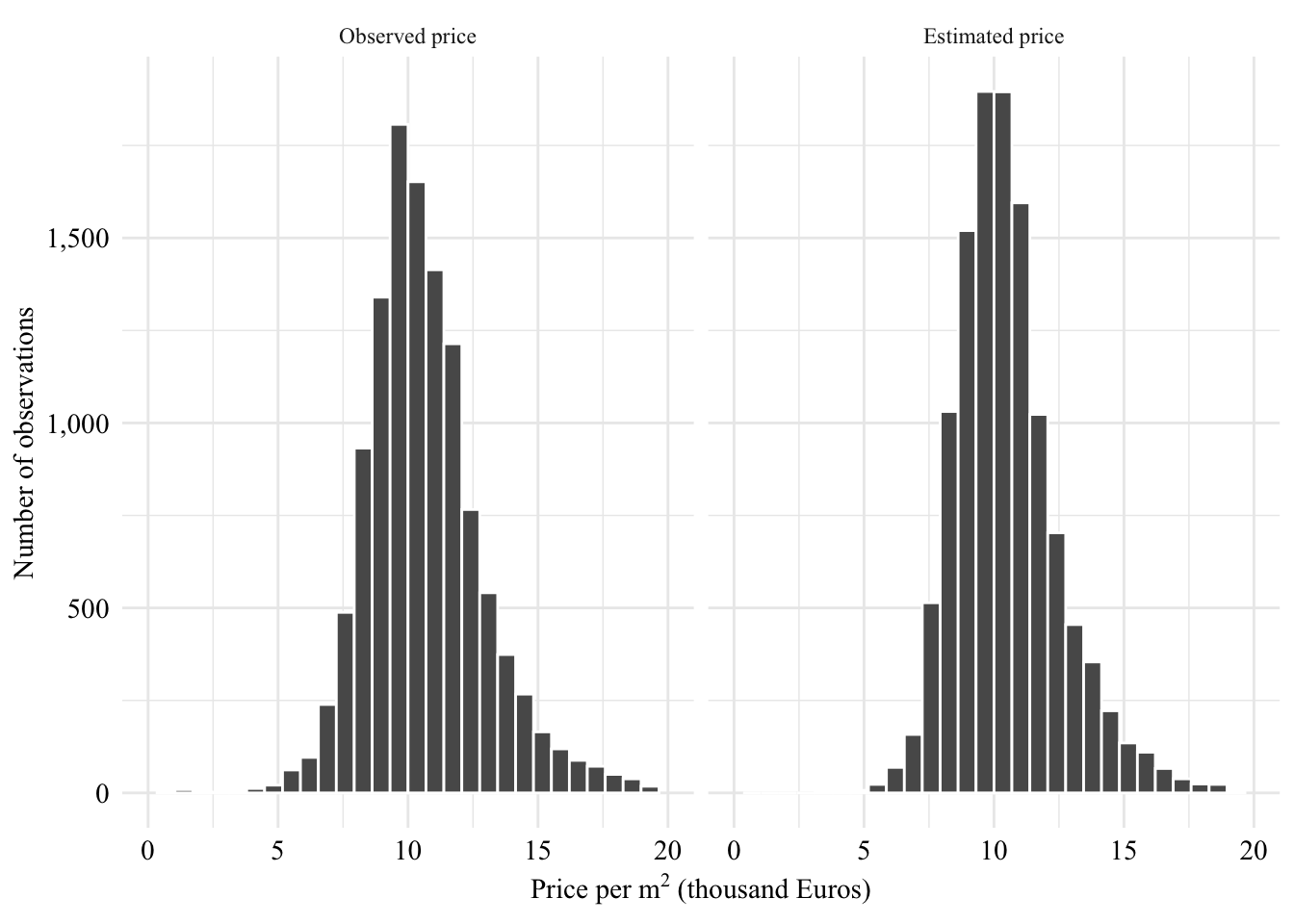
We have access to both the estimated price \(\hat{Z}\) of the underlying property and realized net sale price \(Z\). We also have access to the approximate location and amount of square meters (\(m^2\)) of the property.

We restrict our observations to cases where all the information is available.

data_immo_all <- 
  base_finale |> 
  as_tibble() |> 
  mutate(CODE_IRIS = as.character(iris_cog)) |> 
  mutate(difference_total = contract_final_net_price - backtest_estima) |> 
  mutate(pm2_estimated = backtest_estima/arrea_carrez) |> 
  mutate(difference_pm2 = pm2 - pm2_estimated) |> 
  select(-c(X))
nrow(data_immo_all)

[1] 25675

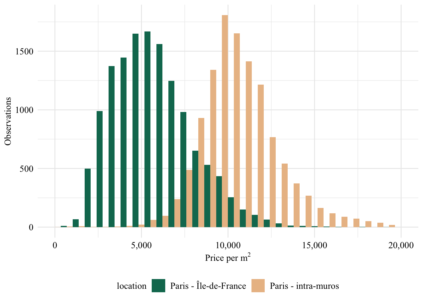
There are 25,675 observation in the dataset. Let us have a look at the number of observations depending on the city. The dataset encompasses data from Paris intra-muros and from other cities within the French departement `Île-de-France’.

data_immo_all <- data_immo_all |> mutate(
  location_city = ifelse(
    city_name == "Paris", 
    yes = "Paris - intra-muros", no = "Paris - Île-de-France")
)

data_immo_all |> count(location_city)

# A tibble: 2 × 2
  location_city             n
  <chr>                 <int>
1 Paris - intra-muros   11906
2 Paris - Île-de-France 13769

Let us visualize the distribution of prices per square meter by location.

Display the codes used to create the Figure.

ggplot(
  data = data_immo_all,
  mapping = aes(x = pm2, fill = location_city)) +
  geom_histogram(position = "dodge") +
  scale_fill_manual(
    "location",
    values = c(
      "Paris - Île-de-France" = colors_[3], 
      "Paris - intra-muros" = colors_[2])
    ) +
  scale_x_continuous(
    labels = scales::label_comma(), 
    limits = c(0, 20000)
  ) +
  labs(x = latex2exp::TeX("Price per $m^2$"), y = "Observations") +
  global_theme() +
  theme(legend.position = "bottom")

Figure 1.1: Price per square meter in different areas of our data. Paris intra-muros refers to the 20 arrondissements that constitute the core of the city, Ile de France refers to the remaining metropolitan area.

We restrict ourselves to Paris intra-muros.

data_immo <- data_immo_all |> 
  filter(city_name == "Paris")
nrow(data_immo)

[1] 11906

This leaves us with 11,906 cases. The range of the sale agreement date is:

range(data_immo$sale_agreement_date)

[1] "2019-01-01" "2019-12-31"

We use the prices per \(m^2\) to normalize the errors by property size.

Display the codes used to create the Figure.

ggplot(
  data = data_immo |> select(pm2, pm2_estimated) |> 
    pivot_longer(cols = c(pm2, pm2_estimated)) |> 
    mutate(
      name = factor(
        name, 
        levels = c("pm2", "pm2_estimated"), 
        labels = c("Observed price", "Estimated price")
      )
    ),
  mapping = aes(x = value)
) +
  geom_histogram(position = "identity", colour = "white") +
  facet_wrap(~name) +
  labs(
    x = latex2exp::TeX("Price per $m^2$ (thousand Euros)"),
    y = "Number of observations"
  ) +
  scale_x_continuous(
    label = scales::label_comma(scale = 1/1000), 
    limits = c(0, 20000)
  ) +
  scale_y_continuous(label = scales::label_comma()) +
  global_theme()

`stat_bin()` using `bins = 30`. Pick better value with `binwidth`.

Warning: Removed 124 rows containing non-finite values (`stat_bin()`).

Warning: Removed 4 rows containing missing values (`geom_bar()`).

Figure 1.2: Distribution of observed and estimated prices.

Let us also create a table with basic summary statistics for the price variables. First, we add labels to the columns of interest here.

data_immo <- data_immo |> 
  labelled::set_variable_labels(
    pm2 = "Observed Price per square meter",
    pm2_estimated = "Estimated Price per square meter"
  )

Table 1.1 shows standard statistics for both the observed and the estimated price.

Display the codes to create the Table.

data_immo |> 
  tbl_summary(
    include = c("pm2", "pm2_estimated"),
    type = all_continuous() ~ "continuous2",
    statistic = list(
      all_continuous() ~ c("{mean} ({sd})", "{median} ({p25}, {p75})"),
      all_categorical() ~ "{n} ({p}%)"),
    digits = list(
      all_continuous() ~ 2,
      all_categorical() ~ 0
    )
  ) |> 
  modify_header(label ~ "**Variable**") |>
  add_stat_label(
    label = list(
      all_continuous() ~ c("Mean (std)", "Median (Q1, Q3)"),
      all_categorical() ~ "n (%)"
    )
  )

Table 1.1:

Descriptive statistics on prices.

Variable	N = 11,906
Observed Price per square meter
Mean (std)	10,784.21 (3,563.00)
Median (Q1, Q3)	10,387.07 (9,200.00, 11,852.03)
Estimated Price per square meter
Mean (std)	10,537.50 (2,408.10)
Median (Q1, Q3)	10,255.28 (9,172.82, 11,506.41)

Let us remove outliers with a price per square meter of over €20,000 and observations from mostly commercial areas.

data_immo <- 
  data_immo |> 
  filter(pm2 <= 20000)

In all, we then have access to 11,812 observations after these basic cleaning steps.

1.3 IRIS

Our Data contains geospatial information, aggregated at the IRIS (Ilots Regroupés pour l’Information Statistique) level, a statistical unit defined and published by the French National Institute of Statistics and Economic Studies.¹ The city of Paris is divided into 20 arrondissements. Each IRIS located in Paris belongs to a single arrondissement.

Tip

Three types of IRIS are distinguished:

• Residential IRIS: their population generally ranges between 1,800 and 5,000 inhabitants. They are homogeneous in terms of housing type, and their boundaries are based on major breaks in the urban fabric (main roads, railways, watercourses, …).

• The IRIS for economic activity: they bring together more than 1,000 employees and have at least twice as many salaried jobs as resident population;

• Miscellaneous IRIS: these are large, specific, sparsely populated areas with significant surface areas (amusement parks, port areas, forests, …).

Source: Limites IRIS - Descriptif de contenu

The total number of IRIS is:

length(unique(data_immo$iris_name))

[1] 880

To plot maps, we first need to get a Parisian map. We use the `Contours… IRIS®’ shapefile from géoservices (édition 2023).

shapes_iris <- str_c(
  "../data/geo/CONTOURS-IRIS_3-0__SHP__FRA_2023-01-01/CONTOURS-IRIS/",
  "1_DONNEES_LIVRAISON_2023-09-00134/CONTOURS-IRIS_3-0_SHP_LAMB93_FXX-2023"
  ) |> 
  sf::st_read(layer="CONTOURS-IRIS", quiet = TRUE)

We extract the Seine River for better looking maps:

shapes_seine <- 
  shapes_iris |> 
  filter(grepl('Paris ', NOM_COM)) |> 
  filter(grepl('Seine ', NOM_IRIS))

To display the Seine River with a single contour, let us create an union of all the polygons that define it:

shapes_seine <- 
  shapes_seine |> 
  summarise(
    geo_ = st_union(geometry)
  )

Let us focus only on Paris intra-muros:

shapes_paris <- 
  shapes_iris |> 
  filter(grepl('Paris ', NOM_COM)) |> 
  mutate(size_poly = as.numeric(st_area(geometry))) |> 
  filter(size_poly < 1840733.0)

Let us save these maps objects for later use.

save(shapes_paris, shapes_seine, file = "../data/shapes.rda")

Let us also export a table with all the IRIS codes in each arrondissement.

aggregation_arrond <- 
  shapes_paris |> 
  select(NOM_COM, CODE_IRIS) |> 
  st_drop_geometry() |> 
  as_tibble() |> 
  write_csv('../data/geo/aggregation_arrond.csv')

1.4 Wealth Level per IRIS

The welth level per IRIS comes from the `Revenus, pauvreté et niveau de vie en 2020 (Iris)’ distributed by the National Institute of Statistics and Economic Studies (INSEE). The data can be downloaded free of charge at the following addreess: https://www.insee.fr/fr/statistiques/7233950#consulter.

data_income <- read_delim(
  str_c(
    "../data/econ/", 
    "BASE_TD_FILO_DISP_IRIS_2020_CSV/BASE_TD_FILO_DISP_IRIS_2020.csv"
  ),
  delim = ";",
  escape_double = FALSE,
  trim_ws = TRUE
)

The median income per IRIS can easily be computed.

median_inc_data <- 
  data_income |> 
  select(CODE_IRIS = IRIS, DISP_MED20) |> 
  mutate(DISP_MED20 = as.numeric(DISP_MED20))

Warning: There was 1 warning in `mutate()`.
ℹ In argument: `DISP_MED20 = as.numeric(DISP_MED20)`.
Caused by warning:
! NAs introduced by coercion

head(median_inc_data)

# A tibble: 6 × 2
  CODE_IRIS DISP_MED20
  <chr>          <dbl>
1 010040101      19450
2 010040102      17910
3 010040201      20210
4 010040202      24870
5 010330102      19810
6 010330103      23770

Note

A choropleth map with smoothed values is shown in Section 2.6 in Chapter 2.

From the Parisian map, we extract some information at the IRIS level: the name of the arrondissement (NOM_COM), the name of the IRIS (NOM_IRIS), and the type of IRIS (TYP_IRIS).

iris_supplementary_data <- 
  shapes_paris |> 
  as_tibble() |> 
  select(CODE_IRIS, NOM_COM, NOM_IRIS, TYP_IRIS)

This information can be added to the real estate data. We will also add income data at the IRIS level in the dataset and define a new categorical variable: income_class which takes three values:

• "rich" if the income in the IRIS is larger or equal to €35,192,
• "poor" if the income in the IRIS is lower or equal to €20,568,
• "others" otherwise.

data_immo <- 
  data_immo |> 
  # Reduce to Parisan data
  inner_join(iris_supplementary_data, by = "CODE_IRIS") |> 
  left_join(
    data_income |> 
      select(CODE_IRIS = IRIS, median_income = DISP_MED20) |> 
      mutate(median_income = as.numeric(median_income)),
    by = "CODE_IRIS"
  ) |> 
  mutate(
    income_class = if_else(
      median_income >= 35192,
      'rich', 
      if_else(median_income <= 20568, 'poor', 'others')
    )
  )

Warning: There was 1 warning in `mutate()`.
ℹ In argument: `median_income = as.numeric(median_income)`.
Caused by warning:
! NAs introduced by coercion

1.5 Export Data

We restrict ourselves to the residential IRIS (type "H") and to sales where both the estimated and the observed price per square meter was below 20,000.

data_clean_all <- 
  data_immo |> 
  filter(TYP_IRIS == 'H')  |> 
  filter(pm2_estimated < 20000) |> 
  filter(pm2 < 20000) 

Then, we save the table for later use.

save(data_clean_all, file = "../data/data_clean_all.rda")
write_csv(data_clean_all, file = "../data/data_clean_all.csv")

---

1. For more information on IRIS, refer to INSEE.