4  Fairness

Display the setting codes

# Required packages----
library(tidyverse)
library(lubridate)
library(gtsummary)
library(labelled)
library(sf)
library(showtext)
library(extrafont)
library(wesanderson)

# Graphs----
font_main = font_title = 'Times New Roman'
extrafont::loadfonts(quiet = T)
face_text='plain'
face_title='plain'
size_title = 14
size_text = 11
legend_size = 11

global_theme <- function() {
  theme_minimal() %+replace%
    theme(
      text = element_text(family = font_main, size = size_text, face = face_text),
      legend.text = element_text(family = font_main, size = legend_size),
      axis.text = element_text(size = size_text, face = face_text), 
      plot.title = element_text(
        family = font_title, 
        size = size_title, 
        hjust = 0.5
      ),
      plot.subtitle = element_text(hjust = 0.5)
    )
}

# Colours
colors_ <- wes_palette('Rushmore1')
col_seine <- "#2140A3"

In this chapter, we mention two types of fairness evaluation:

1. Demographic Parity (Calders, Kamiran, and Pechenizkiy (2009)) (DP): where the objective is the independence of the predictive model from the sensitive attribute,
2. Equalized Odds (Hardt, Price, and Srebro (2016)) (EO): where the objective is independence conditional on all values of the label space.

However, we will compute the Equalized Odds only.

4.1 Background

Recall that our objective is to predict outcomes (prices) within an ordered set \(\mathcal{Y} := [K] = \{1, \ldots, K\}\). We thus face a multi-class classification framework. We use definitions of fairness that are suitable in this framework (see, e.g., Alghamdi et al. (2022) or Denis et al. (2021)).

4.1.1 Demographic Parity (DP)

Let \(\hat{Y}\) be the output of the predictive model \(h\in\mathcal{H}\) defined on \(\mathcal{X}\). From the algorithmic fairness literature, the (empirical) unfairness under DP is defined as follows:

Fairness under Demographic Parity

The unfairness under DP of a classifier \(h\) is quantified by \[ \mathcal{U}_{DP}(h) := \max_{a\in\mathcal{A}, k\in[K]} \left|\, \hat{\mathbb{P}}(\hat{Y} = k | ±\, A = a) - \hat{\mathbb{P}}(\hat{Y} = k)\, \right|\enspace, \]

where (A ) with ( := [M] = {1, , M}) is a discrete group representing specific geographic locations, which constitutes our sentitive attribute.

A model \(h\) is called (empirically) exactly fair under DP i.f.f. \(\mathcal{U}_{DP}(h) = 0\).

When the label \(Y\) is assumed to be unbiased, there emerges a preference for a more nuanced measure of unfairness. Specifically, DP may hinder the realization of an ideal prediction scenario, such as granting loans precisely to those who are unlikely to default.

4.1.2 Equalized Odds (EO)

We assume knowledge of the true and unbiased label \(Y\). The fairness measure under EO is defined as follows:

Fairness under Equalized Odds

The unfairness under EO of a classifier \(h\) is quantified by \[ \mathcal{U}_{EO}(h) := \max_{a\in\mathcal{A}, k, k'\in[K]} \left|\,\hat{\mathbb{P}}(\hat{Y} = k |Y \, = k', \,A = a) - \hat{\mathbb{P}}(\hat{Y} = k | \,Y = k'\,)\right|\enspace. \tag{4.1}\]

A model \(h\) is called (empirically) fair under EO i.f.f. \(\mathcal{U}_{EO}(h) = 0\).

In R, we define the eo_measure() function to compute component of the Equalized Odds formula, for a given protected group \(a\).

#' Calculate Equalized Odds Metrics
#' 
#' @param obs_name name of the variable with observed values in the data
#' @param pred_name name of the variable with predicted values in the data
#' @param quantile_cutoffs quantile cutoffs to use to partition observed and 
#'   predicted values
#' @param group_1 CODE_IRIS belonging to the group of interest ($a$)
#' @param baseline_data data with all the observations
#' 
#' @returns a tibble where each row corresponds to a combination of levels of
#'   the predicted value ($k$, column `quant_predicted`) and the observed 
#'   value ($k'$, column `quant_observed`). For each row, the column 
#'   `value_diff` gives $\hat{P}(\hat{Y} = k | Y = k', A=a) -$ 
#'   $\hat{P}(\hat{Y} = k | Y = k')$ ()
eo_measure <- function(obs_name = "pm2",
                       pred_name = "pm2_estimated",
                       quantile_cutoffs,
                       group_1,
                       baseline_data){
  
  # Assign each bin (based on quantile_cutoffs) to the observed and to the
  # predicted values
  data <- 
    baseline_data |> 
    mutate(
      cut_observed = cut(
        !!sym(obs_name), 
        quantile_cutoffs, 
        c(1:(length(quantile_cutoffs) - 1))
      )
    ) |> 
    mutate(
      cut_predictions = cut(
        !!sym(pred_name), 
        quantile_cutoffs, 
        c(1:(length(quantile_cutoffs) - 1))
      )
    )
  
  retainer_1 <- c()
  retainer_2 <- c()
  value_retainer <- c()
  # Looping over classes (k)
  for (level_1 in c(1:(length(quantile_cutoffs) - 1))) {
    # Looping over classes (k')
    for (level_2 in c(1:(length(quantile_cutoffs) - 1))) {
      
      # Identify whether Y==k & \hat{Y} == k'
      bucket_tmp <- 
        data |> 
        select(
          CODE_IRIS, !!obs_name, !!pred_name, cut_observed, cut_predictions
        ) |> 
        mutate(
          in_bucket = if_else(
            cut_observed == level_1 & cut_predictions == level_2, 1, 0)
        )
      
      # \hat{P}(\hat{Y} = k | Y = k')
      p_average <- 
        bucket_tmp |> 
        pull(in_bucket)|> 
        mean(na.rm = T)
      
      # \hat{P}(\hat{Y} = k | Y = k', A=a)
      p_special <- 
        bucket_tmp|> 
        filter(CODE_IRIS %in% group_1) |> 
        pull(in_bucket) |> 
        mean(na.rm = T)
      
      # Store this (we need to find the max among those at the end of the loop)
      value_tmp <- abs(p_special - p_average)
      
      value_retainer <- c(value_retainer, value_tmp)
      retainer_1 <- c(retainer_1, level_1)
      retainer_2 <- c(retainer_2, level_2)
    }
  }
  
 tibble(
    value_diff = value_retainer, 
    quant_observed = retainer_1, 
    quant_estimated = retainer_2
  )
}

4.2 Load Data

Let us load the real estate data that were cleaned in Section 1.5 in Chapter 1.

load("../data/data_clean_all.rda")

Let us also load the Parisian map saved in Section 1.3 from Chapter 1.

load("../data/shapes.rda")

In Section 2.3 from Chapter 2, we computed the minimum distance from one iris to another, considering distances up to 30. We will also need this informations.

neighbours_all <- read_csv('../data/neighbours/all_neighbours_paris.csv')

4.3 Equalized Odds

Let us compute the Equalized Odds, using the eo_measure() function. We will consider the predicted prices as well as some randomly drawn values. In each case, we will compute the Equalized Odds.

4.3.1 EO with Predicted Prices

We need to define a partitioning of the data. We consider the quantiles of the observed price as the cutoffs. We will make the number of neighbors used to spatially smooth data vary. But before doing so, we would like to spend some time with a small example.

limits_quants <- 
  data_clean_all |> 
  pull(pm2) |> 
  quantile(seq(0,1,0.2)) |> 
  unname()
limits_quants

[1]    11.97183  8893.48074  9941.87479 10829.77717 12122.78446 19994.28735

We want to examine the variation of the EO depending on the aggregation considered. Let us consider the immediate neighbors to begin with.

num_neigh <- 1

We will focus on two IRIS: Montmartre and Champs-de-Mars (see Figure 2.4 from Chapter 2 to locate those two IRIS on the Parisian map). We extract the IRIS codes of those two IRIS.

want_montmartre <- 
  neighbours_all |> 
    filter(from_iris == '751093503') |> 
    filter(distance <= num_neigh) |> 
    pull(to_iris)
want_mars <- 
  neighbours_all |> 
    filter(from_iris == '751072812') |> 
    filter(distance <= num_neigh) |> 
    pull(to_iris)

Then, we can compute the components of the EO formula, for each combination of \(k\) and \(k'\) (see Equation 4.1).

re_mont <- eo_measure(
  obs_name = "pm2",
  pred_name = "pm2_estimated",
  quantile_cutoffs = limits_quants, 
  group_1 = want_montmartre, 
  baseline_data = data_clean_all
)
re_mont

# A tibble: 25 × 3
   value_diff quant_observed quant_estimated
        <dbl>          <int>           <int>
 1   0.119                 1               1
 2   0.0462                1               2
 3   0.0214                1               3
 4   0.000272              1               4
 5   0.00242               1               5
 6   0.0438                2               1
 7   0.0455                2               2
 8   0.0115                2               3
 9   0.0327                2               4
10   0.00260               2               5
# ℹ 15 more rows

Let us extract, among these elements, the maximum value:

eo_mont <- 
  re_mont |> 
   arrange(desc(value_diff)) |> 
    head(1) |> 
    pull(value_diff)

We do the same for Champs de Mars:

re_mars <- eo_measure(
  obs_name = "pm2",
  pred_name = "pm2_estimated",
  quantile_cutoffs = limits_quants, 
  group_1 = want_mars, 
  baseline_data = data_clean_all
)

eo_mars <- 
  re_mars |> 
   arrange(desc(value_diff)) |> 
    head(1) |> 
    pull(value_diff)
eo_mars

[1] 0.7387795

Now, let us encompass the previous code inside a loop to consider different spatial aggregation levels.

all_eo_mars <- c()
all_eo_mont <- c()
for (num_neigh in c(1:9)) {
  # Montmartre----
  want_montmartre <- 
    neighbours_all |> 
    filter(from_iris == '751093503') |> 
    filter(distance <= num_neigh) |> 
    pull(to_iris)
  
  re_mont <- eo_measure(
    obs_name = "pm2",
    pred_name = "pm2_estimated",
    quantile_cutoffs = limits_quants, 
    group_1 = want_montmartre, 
    baseline_data = data_clean_all
  )
  
  eo_mont_value_tmp <- 
    re_mont |> 
    arrange(desc(value_diff)) |> 
    head(1) |> 
    pull(value_diff)
  
  all_eo_mont <- c(all_eo_mont, eo_mont_value_tmp)

  # Champs-de-Mars----
  want_mars <- 
    neighbours_all %>% 
    filter(from_iris == '751072812') |> 
    filter(distance <= num_neigh) |> 
    pull(to_iris)
  
  re_mars <- eo_measure(
    obs_name = "pm2",
    pred_name = "pm2_estimated",
    quantile_cutoffs = limits_quants, 
    group_1 = want_mars, 
    baseline_data = data_clean_all
  )
  
  eo_mars_value_tmp <- 
    re_mars |> 
    arrange(desc(value_diff)) |> 
    head(1) |> 
    pull(value_diff)
  
  all_eo_mars <- c(all_eo_mars, eo_mars_value_tmp)
}

We can then store the EO computed for Montmartre and for Champs-de-Mars, depending on the number of neighbors considered.

data_eo_res <- tibble(
  neighbours = c(1:9),
  all_mars = all_eo_mars, 
  all_nine = all_eo_mont, 
)
data_eo_res

# A tibble: 9 × 3
  neighbours all_mars all_nine
       <int>    <dbl>    <dbl>
1          1   0.739    0.119 
2          2   0.449    0.107 
3          3   0.290    0.106 
4          4   0.184    0.0750
5          5   0.178    0.0421
6          6   0.165    0.0318
7          7   0.158    0.0239
8          8   0.133    0.0202
9          9   0.0911   0.0279

4.3.2 EO with Random Values

Let us now turn to the evaluation of EO where we no longer use the predicted prices, but rather draw random values, in a similar fashion to what was done in Section 3.5.2 from Chapter 3.

We define a function, eo_measure_random(){R} that will compute the EO based on random values for the predicted prices. This function works as follows:

1. Simulation of observed prices:

• we draw values from a Uniform distribution, where the bounds are the price range from the estimated prices

#' Calculate Equalized Odds Metrics using randomly drawn predicted values
#' 
#' @param obs_name name of the variable with observed values in the data
#' @param pred_name name of the variable with predicted values in the data
#' @param quantile_cutoffs quantile cutoffs to use to partition observed and 
#'   predicted values
#' @param baseline_data data with all the observations
#' 
#' @returns a list with two elements:
#'  - `data_random` the data set with randomly drawn values for the prediction
#'  - `metrics`: #' a tibble where each row corresponds to a combination of levels of
#'   the predicted value ($k$, column `quant_predicted`) and the observed 
#'   value ($k'$, column `quant_observed`). For each row, the column 
#'   `value_diff` gives $\hat{P}(\hat{Y} = k | Y = k', A=a) -$ 
#'   $\hat{P}(\hat{Y} = k | Y = k')$ ()
eo_measure_random <- function(obs_name = "pm2",
                              pred_name = "pm2_estimated",
                              quantile_cutoffs,
                              baseline_data) {
  
  # Simulate estimated prices----
  
  # bounds for the Uniform
  range_prices <- 
    baseline_data |> 
    pull(!!pred_name) |> 
    range()
  # No values to draw
  rand_obs <- nrow(baseline_data)
  # Draw values
  random_prices <- runif(rand_obs, range_prices[1], range_prices[2])
  
  # Replace observed values by random ones
  data_random <- baseline_data |>  
    mutate(!!pred_name := !!random_prices)
  
  # Assign each bin (based on quantile_cutoffs) to the observed and to the
  # 'predicted' values (random data)
  data_random <- data_random |> 
    mutate(
      cut_observed = cut(
        !!sym(obs_name),
        quantile_cutoffs, 
        c(1:(length(quantile_cutoffs) - 1))
      )
    )|> 
    mutate(
      cut_predictions = cut(
        !!sym(pred_name),
        quantile_cutoffs, 
        c(1:(length(quantile_cutoffs) - 1))
      )
    )
  
  # Assign each bin (based on quantile_cutoffs) to the observed and to the
  # predicted values (baseline data)
  data <- baseline_data |> 
    mutate(
      cut_observed = cut(
        !!sym(obs_name),
        quantile_cutoffs, 
        c(1:(length(quantile_cutoffs) - 1))
      )
    )|> 
    mutate(
      cut_predictions = cut(
        !!sym(pred_name),
        quantile_cutoffs, 
        c(1:(length(quantile_cutoffs) - 1))
      )
    )
  
  
  retainer_1 <- c()
  retainer_2 <- c()
  value_retainer <- c()
  # Looping over classes (k)
  for (level_1 in c(1:(length(quantile_cutoffs) - 1))) {
    # Looping over classes (k)
    for (level_2 in c(1:(length(quantile_cutoffs) - 1))) {
      
      
      ## Identify whether Y==k & \hat{Y} == k' (baseline data)
      bucket_tmp <- 
        data |> 
        select(
          CODE_IRIS, !!obs_name, !!pred_name, cut_observed, cut_predictions
        ) |> 
        mutate(
          in_bucket = if_else(
            cut_observed == level_1 & cut_predictions == level_2, 1, 0)
        )
      
      # (random data)
      bucket_random_tmp <- 
        data_random |> 
        select(
          CODE_IRIS, !!obs_name, !!pred_name, cut_observed, cut_predictions
        ) |> 
        mutate(
          in_bucket = if_else(
            cut_observed == level_1 & cut_predictions == level_2, 1, 0)
        )
      
      ## \hat{P}(\hat{Y} = k | Y = k') (on baseline data)
      p_average <- bucket_tmp |> 
        pull(in_bucket) |> 
        mean(na.rm = T)
      
      ## \hat{P}(\hat{Y} = k | Y = k', A=a) (on random data)
      p_special <-
        bucket_random_tmp |> 
        pull(in_bucket) |> 
        mean(na.rm = T)
      
      # Store this (we need to find the max among those at the end of the loop)
      value_tmp <- abs(p_special - p_average)
      
      value_retainer <- c(value_retainer, value_tmp)
      retainer_1 <- c(retainer_1, level_1)
      retainer_2 <- c(retainer_2, level_2)
    }
  }
  
  list(
    data_random = data_random,
    metrics = tibble(
      value_diff = value_retainer, 
      quant_observed = retainer_1, 
      quant_estimated = retainer_2
    )
  )
}

We compute the components of the EO formula:

re <- eo_measure_random(
  obs_name = "pm2",
  pred_name = "pm2_estimated",
  quantile_cutoffs = limits_quants, 
  baseline_data = data_clean_all
)
data_random <- re$data_random
re$metrics

# A tibble: 25 × 3
   value_diff quant_observed quant_estimated
        <dbl>          <int>           <int>
 1    0.0500               1               1
 2    0.0412               1               2
 3    0.00860              1               3
 4    0.00707              1               4
 5    0.0927               1               5
 6    0.0205               2               1
 7    0.0741               2               2
 8    0.0373               2               3
 9    0.00385              2               4
10    0.0948               2               5
# ℹ 15 more rows

Then, among these elements, we extract the maximum value:

random_eo <- 
  re$metrics |> 
  arrange(desc(value_diff)) |> 
  head(1) |> 
  pull(value_diff)
random_eo

[1] 0.09482473

4.4 Visualization of the Results

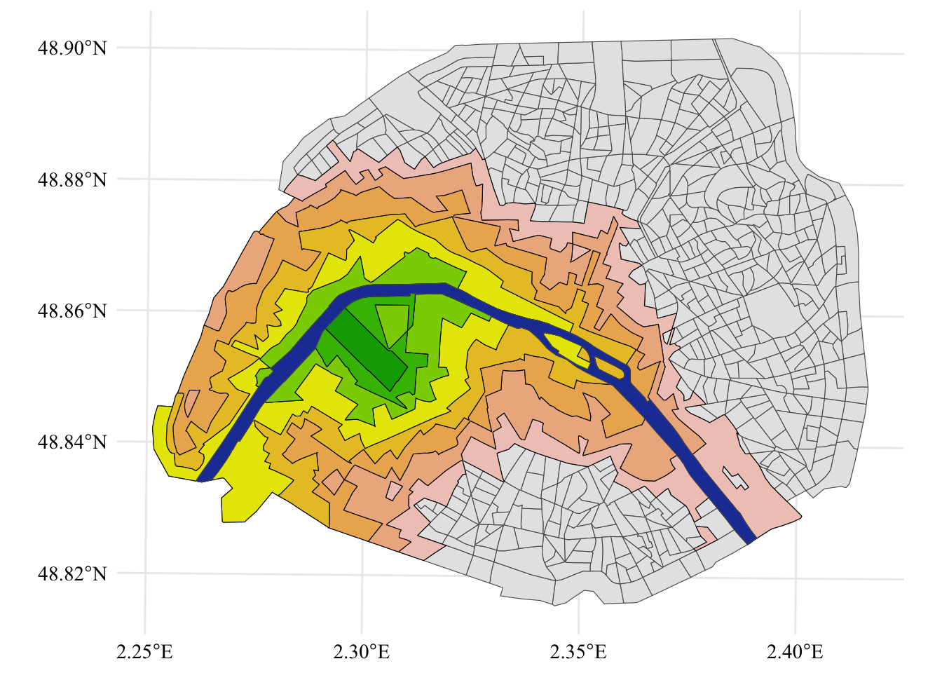
Let us now visualize how the EO metrics expands as the level of spatial aggregation increases, starting from the two IRIS regions corresponding to Champs-de-Mars and Montmartre.

Let us isolate each level of neighbors for Champs-de-Mars and Montmartre. The following loop will create objects named full_champ_1 (immediate neighbors), full_champ_2 (neighbors of neighbors), etc. up to full_champ_8

for (num_neigh in 1:8) {
  full_champs_current <- 
    shapes_paris |> 
    left_join(
      neighbours_all |> 
        filter(from_iris == '751072812') |> 
        filter(distance == !!num_neigh) |> 
        mutate(is_neigh = 'yes') |> 
        mutate(CODE_IRIS = as.character(to_iris)) |> 
        select(CODE_IRIS, is_neigh),
      by = "CODE_IRIS"
    ) |> 
    mutate(is_neigh = if_else(is.na(is_neigh), 'no', 'yes')) |> 
    group_by(is_neigh) |> 
    summarise(comb_lev_1 = st_union(geometry)) |> 
    filter(is_neigh == 'yes')
  
  assign(str_c("full_champ_", num_neigh), value = full_champs_current)
}

Let us do something similar for Montmartre.

for (num_neigh in 1:8) {
  full_mont_current <- 
    shapes_paris |> 
    left_join(
      neighbours_all |> 
        filter(from_iris == '751093503') |> 
        filter(distance == !!num_neigh) |> 
        mutate(is_neigh = 'yes') |> 
        mutate(CODE_IRIS = as.character(to_iris)) |> 
        select(CODE_IRIS, is_neigh),
      by = "CODE_IRIS"
    ) |> 
    mutate(is_neigh = if_else(is.na(is_neigh), 'no', 'yes')) |> 
    group_by(is_neigh) |> 
    summarise(comb_lev_1 = st_union(geometry)) |> 
    filter(is_neigh == 'yes')
  
  assign(str_c("full_mont_", num_neigh), value = full_mont_current)
}

We will use the following colors to identify the distance for the neighbors:

colors_want <- terrain.colors(9)

Champs-de-Mars

Display the codes used to create the Figure.

map_champ <- 
  shapes_paris |> 
  mutate(centroid = st_centroid(geometry)) |> 
  ggplot() +
  geom_sf() + 
  geom_sf(data = full_champ_8, fill = colors_want[8], color = 'black') + 
  geom_sf(data = full_champ_7, fill = colors_want[7], color = 'black') + 
  geom_sf(data = full_champ_6, fill = colors_want[6], color = 'black') + 
  geom_sf(data = full_champ_5, fill = colors_want[5], color = 'black') + 
  geom_sf(data = full_champ_4, fill = colors_want[4], color = 'black') + 
  geom_sf(data = full_champ_3, fill = colors_want[3], color = 'black') + 
  geom_sf(data = full_champ_2, fill = colors_want[2], color = 'black') + 
  geom_sf(data = full_champ_1, fill = colors_want[1], color = 'black') + 
  geom_sf(data = shapes_seine, fill = col_seine) + 
  global_theme() +
  theme(legend.position = 'bottom') + 
  labs(fill = 'EO measure')

map_champ

Figure 4.1: Champs de Mars and its IRIS neighbors.

Montmartre

Display the codes used to create the Figure.

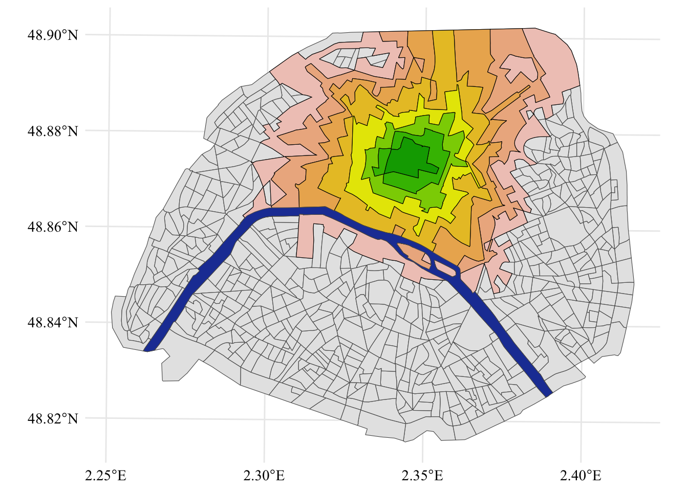
map_mont <- 
  shapes_paris |> 
  mutate(centroid = st_centroid(geometry)) |> 
  ggplot() +
  geom_sf() + 
  geom_sf(data = full_mont_8, fill = colors_want[8], color = 'black') + 
  geom_sf(data = full_mont_7, fill = colors_want[7], color = 'black') + 
  geom_sf(data = full_mont_6, fill = colors_want[6], color = 'black') + 
  geom_sf(data = full_mont_5, fill = colors_want[5], color = 'black') + 
  geom_sf(data = full_mont_4, fill = colors_want[4], color = 'black') + 
  geom_sf(data = full_mont_3, fill = colors_want[3], color = 'black') + 
  geom_sf(data = full_mont_2, fill = colors_want[2], color = 'black') + 
  geom_sf(data = full_mont_1, fill = colors_want[1], color = 'black') + 
  geom_sf(data = shapes_seine, fill = col_seine) + 
  global_theme() +
  theme(legend.position = 'bottom') + 
  labs(fill = 'EO measure')

map_mont

Figure 4.2: Montmartre and its IRIS neighbors.

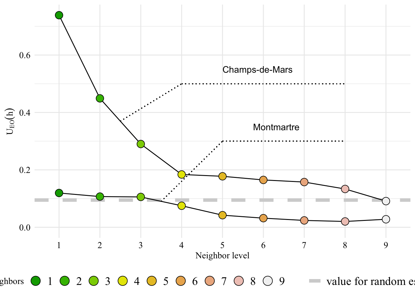
Now, let us plot the EO measure as a function of the neighbor level.

Display the codes used to create the Figure.

lineplot_eo <- 
  data_eo_res |> 
  select(
    neighbors = neighbours, 
    `Champs de Mars` = all_mars, 
    Montmartre = all_nine
  ) |> 
  mutate(neighbors = as.character(neighbors)) |> 
  pivot_longer(
    cols = c(`Champs de Mars`:Montmartre),
    names_to = "IRIS region", values_to = "value"
  ) %>% 
  ggplot(data = .) + 
  geom_hline(
    mapping = aes(
      yintercept = random_eo, 
      color = 'value for random estimation'
    ), 
    lwd = 2, 
    lty = 'dashed'
  ) +
  geom_line(
    mapping = aes(
      x = neighbors,
      y = value, 
      group = `IRIS region`
    )
  ) + 
  geom_point(
    mapping = aes(
      x = neighbors,
      y = value,
      fill = neighbors
    ),
    pch = 21,
    size = 4
  ) + 
  # Champs-de-Mars
  geom_segment(
    x = 2.5,
    y = (data_eo_res$all_mars[2] + data_eo_res$all_mars[3]) / 2,
    xend = 4,
    yend = .5,
    lty = 3
  ) +
  geom_segment(
    x = 4,
    y = .5,
    xend = 8,
    yend = .5,
    lty = 3
  ) +
  annotate(
    geom = "text", x = 5, 
    y = .55, 
    label = "Champs-de-Mars",
    hjust = 0
  ) +
  # Montmartre
  geom_segment(
    x = 3.5,
    y = (data_eo_res$all_nine[3] + data_eo_res$all_nine[4]) / 2,
    xend = 5,
    yend = .3,
    lty = 3
  ) +
  geom_segment(
    x = 5,
    y = .3,
    xend = 8,
    yend = .3,
    lty = 3
  ) +
  annotate(
    geom = "text", x = 5.75, 
    y = .35, 
    label = "Montmartre",
    hjust = 0
  ) +
  scale_color_manual(values = c('lightgrey')) + 
  scale_fill_manual(values = colors_want) +
  ylab(latex2exp::TeX(r'($U_{EO}(h)$)')) +
  xlab('Neighbor level') + 
  global_theme() + 
  theme(
    legend.position = 'bottom',
    # legend.box="vertical",
    legend.text = element_text(family = font_main, size = 14)
  ) + 
  guides(fill = guide_legend(override.aes = list(size=5), nrow=1)) + 
  guides(color = guide_legend(title='')) + 
  guides(linetype = guide_legend(title='')) + 
  ylim(c(0,0.739))

lineplot_eo

Figure 4.3: Equalized Odds Measure for Montmartre and Champ-de-Mars.

Let us load the calibration errors computed for those two IRIS, in Section 3.7 in Chapter 3.

load("../data/ece_neighbours_montmartre.rda")
load("../data/ece_neighbours_mars.rda")

Display the codes used to create the Figure.

lineplot_ece <- 
  ece_neighbours_montmartre |> 
  bind_rows(ece_neighbours_mars) |> 
  rename(`IRIS region` = iris_name) |> 
  mutate(neighbors = as.character(neighbours), value = ece) |> 
  ggplot() + 
  geom_hline(
    mapping = aes(
      yintercept = .0262022, # VALUE OBTAINED IN PREVIOUS CHAPTER
      color = 'value for random estimation'
    ), 
    lwd = 2, 
    lty = 'dashed'
  ) +
  geom_line(
    mapping = aes(
      x = neighbors,
      y = ece, 
      group = `IRIS region`,
    )
  ) + 
  geom_point(
    mapping = aes(
      x = neighbors,
      y = value,
      fill = neighbors
    ),
    pch = 21,
    size = 4
  ) + 
  # Champs-de-Mars
  geom_segment(
    x = 1.5,
    y = (ece_neighbours_mars$ece[1] + ece_neighbours_mars$ece[2]) / 2,
    xend = 3,
    yend = .5,
    lty = 3
  ) +
  geom_segment(
    x = 3,
    y = .5,
    xend = 7,
    yend = .5,
    lty = 3
  ) +
  annotate(
    geom = "text", x = 4,
    y = .55,
    label = "Champs-de-Mars",
    hjust = 0
  ) +
  # Montmartre
  geom_segment(
    x = 3.5,
    y = (ece_neighbours_montmartre$ece[3] + ece_neighbours_montmartre$ece[4]) / 2,
    xend = 5,
    yend = .3,
    lty = 3
  ) +
  geom_segment(
    x = 5,
    y = .3,
    xend = 8,
    yend = .3,
    lty = 3
  ) +
  annotate(
    geom = "text", x = 5.75, 
    y = .35, 
    label = "Montmartre",
    hjust = 0
  ) +
  scale_color_manual(values = c('lightgrey')) + 
  scale_fill_manual(values = colors_want) +
  ylab(latex2exp::TeX(r'($U_{ECE}(h)$)')) +
  xlab('Neighbor level') + 
  global_theme() + 
  theme(
    legend.position = 'bottom',
    # legend.box="vertical",
    legend.text = element_text(family = font_main, size = 14)
  ) + 
  guides(fill = guide_legend(override.aes = list(size = 5), nrow = 1)) + 
  guides(color = guide_legend(title = '')) + 
  guides(linetype = guide_legend(title='')) + 
  ylim(c(0,0.739))

lineplot_ece

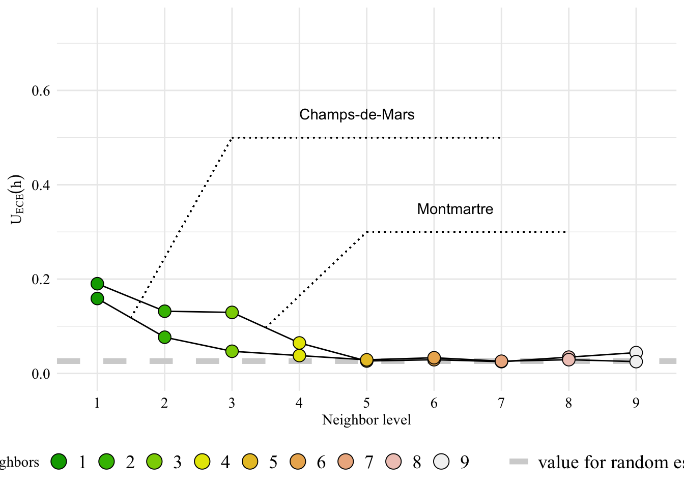
Figure 4.4: Expected Calibration Error Measure for Montmartre and Champ-de-Mars.

4.5 EO on each Arrondissement

Now, we can compute the Equalized Odds metric on each arrondissement. For convenience, let us create a function, calculate_eo_arrond(), that computes EO on a single arrondissement.

#' EO metric for an arrondissement
#' 
#' @param arrond name of the arrondissement
#' @param num_neigh distance of neighbors to include
#' @param obs_name name of the variable with observed values in the data
#' @param pred_name name of the variable with predicted values in the data
#' @param data dataset to use
calculate_eo_arrond <- function(arrond, 
                                num_neigh, 
                                obs_name = "pm2",
                                pred_name = "pm2_estimated",
                                data) {
  
  # Cutoff to partition data
  limits_quants <- 
    data |> 
    pull(!!obs_name) |> 
    quantile(seq(0,1,0.2)) |> 
    unname()
  
  # Extract IRIS in the arrondissement
  want_arrond <- 
    data |> 
    filter(NOM_COM %in% arrond) |> 
    pull(CODE_IRIS) |> 
    unique()
  
  re_arrond <- eo_measure(
    obs_name = obs_name,
    pred_name = pred_name,
    quantile_cutoffs = limits_quants, 
    group_1 = want_arrond, 
    baseline_data = data
  )
  
  ece_arrond <- 
    re_arrond |> 
    arrange(desc(value_diff)) |> 
    head(1) |> 
    pull(value_diff)
  
  ece_arrond
}

All that needs to be done is to loop over the names of the arrondissements.

name_arronds <- unique(data_clean_all$NOM_COM)
name_arronds <- name_arronds[!is.na(name_arronds)]

eo_arrond <- map_dbl(
  .x = name_arronds,
  .f = ~calculate_eo_arrond(
    arrond = .x, 
    num_neigh = 5, 
    obs_name = "pm2", 
    pred_name = "pm2_estimated", 
    data = data_clean_all
  )
)

We can put those values in a tibble:

eo_arrond_tb <- tibble(
  arrondissement = name_arronds,
  ece = eo_arrond
) |> 
  mutate(
    arrondissement = factor(
      arrondissement, 
      levels = str_c(
        "Paris ", 1:20, "e", c("r", rep("", 19)), " Arrondissement")
    )
  ) |> 
  arrange(arrondissement)

The values can be saved:

save(eo_arrond_tb, file = "../data/eo_arrond_tb.rda")

For comparison with the Expected Calibration Error, let us load the results obtained in Section 3.6 in Chapter 3.

load("../data/ece_arrond_tb.rda")

The values are reported in Table 4.1.

Display the codes used to create the Table

ece_arrond_tb |> 
  left_join(
    eo_arrond_tb, by = "arrondissement"
  ) |> 
  knitr::kable(
    booktabs = TRUE, digits = 3,
    col.names = c("Arrondissement", "ECE", "EO")
  )

Table 4.1: Equalized Odds per Arrondissement.

Arrondissement	ECE	EO
Paris 1er Arrondissement	0.188	0.301
Paris 2e Arrondissement	0.097	0.146
Paris 3e Arrondissement	0.126	0.319
Paris 4e Arrondissement	0.116	0.469
Paris 5e Arrondissement	0.131	0.280
Paris 6e Arrondissement	0.126	0.637
Paris 7e Arrondissement	0.170	0.625
Paris 8e Arrondissement	0.157	0.128
Paris 9e Arrondissement	0.120	0.117
Paris 10e Arrondissement	0.132	0.114
Paris 11e Arrondissement	0.136	0.108
Paris 12e Arrondissement	0.102	0.115
Paris 13e Arrondissement	0.052	0.177
Paris 14e Arrondissement	0.089	0.070
Paris 15e Arrondissement	0.072	0.072
Paris 16e Arrondissement	0.055	0.107
Paris 17e Arrondissement	0.096	0.085
Paris 18e Arrondissement	0.029	0.145
Paris 19e Arrondissement	0.078	0.396
Paris 20e Arrondissement	0.088	0.242

Alghamdi, Wael, Hsiang Hsu, Haewon Jeong, Hao Wang, Peter Michalak, Shahab Asoodeh, and Flavio Calmon. 2022. “Beyond Adult and COMPAS: Fair Multi-Class Prediction via Information Projection.” Advances in Neural Information Processing Systems 35: 38747–60.

Calders, T., F. Kamiran, and M. Pechenizkiy. 2009. “Building Classifiers with Independency Constraints.” In IEEE International Conference on Data Mining.

Denis, Christophe, Romuald Elie, Mohamed Hebiri, and François Hu. 2021. “Fairness Guarantee in Multi-Class Classification.” arXiv Preprint arXiv:2109.13642.

Hardt, M., E. Price, and N. Srebro. 2016. “Equality of Opportunity in Supervised Learning.” In Neural Information Processing Systems.