library(tidyverse)
library(mnormt)6 Monte Carlo Simulations
Objectives
In this chapter, we use the same data-generating process described in Chapter 5 and run a series of Monte Carlo experiments. We consider two types of scenarios:
We change the distance between the means of the Gaussian distributions in groups 0 and 1. As this distance increases, the overlap between the two groups decreases.
We let the proportion of individuals in group 0 relative to group 1 vary. This simulates different levels of class imbalance.
Codes for graphical parameters
library(extrafont, quietly = TRUE)
col_group <- c("#00A08A","#F2AD00", "#1b95e0")
colour_methods <- c(
    "OT" = "#CC79A7", "OT-M" = "#009E73",
    "skh" = "darkgray",
    "seq_1" = "#0072B2", "seq_2" = "#D55E00",
    "fairadapt_1" = "#9966FF",
    "fairadapt_2" = "#7CAE00"
  )
colGpe1 <- col_group[2]
colGpe0 <- col_group[1]
colGpet <- col_group[3]
loadfonts(device = "pdf", quiet = TRUE)
font_size <- 20
font_family <- "CMU Serif"

path <- "./figs/"
if (!dir.exists(path)) dir.create(path)

source("../scripts/utils.R")
\[ \definecolor{wongBlack}{RGB}{0,0,0} \definecolor{wongGold}{RGB}{230, 159, 0} \definecolor{wongLightBlue}{RGB}{86, 180, 233} \definecolor{wongGreen}{RGB}{0, 158, 115} \definecolor{wongYellow}{RGB}{240, 228, 66} \definecolor{wongBlue}{RGB}{0, 114, 178} \definecolor{wongOrange}{RGB}{213, 94, 0} \definecolor{wongPurple}{RGB}{204, 121, 167} \definecolor{colGpe1}{RGB}{0, 160, 138} \definecolor{colGpe0}{RGB}{242, 173, 0} \]
6.1 Functions
Let us redefine the function shown in Chapter 5 that will be used to perform the simulations here.
Functions used to generate the data (gen_data()), create counterfactuals with optimal transport (compute_ot_map(), apply_ot_transport()) and sequential transport (sequential_transport_12(), sequential_transport_21()), compute the total causal effect based on (causal_effects_cf())
## Data----

#' @param n0 Number of units in group 0.
#' @param n1 Number of units in group 1.
#' @param mu0 Mean of the two covariates in group 0.
#' @param mu1 Mean of the two covariates in group 1.
#' @param r0 Covariance of the two covariates in group 0.
#' @param r1 Covariance of the two covariates in group 1.
#' @param a Shift parameter for the mean in both groups (default to 1: no shift). Larger values decrease overlap.
#' @param seed Random seed for reproducibility.
gen_data <- function(n0 = 250,
                     n1 = 250,
                     mu0 = -1,
                     mu1 = +1,
                     r0 = +.7,
                     r1 = -.5,
                     a = 1,
                     seed = NULL) {

  if (!is.null(seed)) set.seed(seed)

  a0 <- 3
  a1 <- 2
  a2 <- -1.5
  Mu0 <- rep(mu0, 2)
  Mu1 <- rep(mu1, 2)
  Sig0 <- matrix(c(1, r0, r0, 1), 2, 2)
  Sig1 <- matrix(c(1, r1, r1, 1), 2, 2)

  # Generate covariates for each group
  X0 <- rmnorm(n0, mean = a * Mu0, varcov = Sig0)
  X1 <- rmnorm(n1, mean = a * Mu1, varcov = Sig1)
  # Combine into a single covariate matrix
  X <- rbind(X0, X1)
  # Treatment indicator: 0 for first n0, 1 for next n1
  A <- c(rep(0, n0), rep(1, n1))
  # Random noise for each unit
  E <- rnorm(n0 + n1)

  # Outcomes
  Y0 <- a1 * X[, 1] + a2 * X[, 2] + E
  Y1 <- a1 * X[, 1] + a2 * X[, 2] + a0 + E
  Y <- A * Y1 + (1 - A) * Y0

  df <- tibble(
    X1 = X[, 1],
    X2 = X[, 2],
    A = A,
    Y0 = Y0,
    Y1 = Y1,
    Y  = Y
  )

  df
}

## Optimal Transport----

#' Optimal transport mapping between two Gaussian distributions
#'  (from \eqn{\mathcal{N}(\mu_{\text{source}}, \Sigma_{\text{source}})} to
#'   \eqn{\mathcal{N}(\mu_{\text{target}}, \Sigma_{\text{target}})})
#'
#' @param mu_source Mean vector of the source Gaussian.
#' @param sigma_source Covariance matrix of the source Gaussian.
#' @param mu_target Mean vector of the target Gaussian.
#' @param sigma_target Covariance matrix of the target Gaussian.
compute_ot_map <- function(mu_source, sigma_source, mu_target, sigma_target) {
  sqrt_sigma_source <- sqrtm(sigma_source)
  sqrt_sigma_source_inv <- solve(sqrt_sigma_source)

  inner <- sqrt_sigma_source %*% sigma_target %*% sqrt_sigma_source
  sqrt_inner <- sqrtm(inner)

  A <- sqrt_sigma_source_inv %*% sqrt_inner %*% sqrt_sigma_source_inv

  list(A = A, shift = mu_target - A %*% mu_source)
}

#' Function to apply the transport map to simulated data
#'
#' @param X Observations to transport.
#' @param mapping Optimal transport mapping (from `compute_ot_map()`)?
apply_ot_transport <- function(X, mapping) {
  A <- mapping$A
  shift <- mapping$shift
  t(apply(X, 1, function(x) as.vector(shift + A %*% x)))
}

## Penalized Transport----
#' @param X_source Matrix of observations to transport from the source group.
#' @param X_target Matrix of observations from the target group.
#' @param gamma A regularization parameter (default to 0.1).
transport_regul <- function(X_source,
                            X_target,
                            gamma) {

  X_source <- as.matrix(X_source)
  X_target <- as.matrix(X_target)
  n_source <- nrow(X_source)
  n_target <- nrow(X_target)
  # Uniform weights
  w_source <- rep(1 / n_source, n_source)
  w_target <- rep(1 / n_target, n_target)

  # Pairwise squared Euclidean distance
  cost_mat <- as.matrix(dist(rbind(X_source, X_target)))^2
  C <- cost_mat[1:n_source, (n_source + 1):(n_source + n_target)]

  # Run Sinkhorn with entropic regularization gamma
  skh_res <- T4transport::sinkhornD(
    D = C, p = 2, wx = w_source, wy = w_target, lambda = gamma
  )

  # Extract and normalize plan
  ot_plan_skh <- skh_res$plan
  ot_plan_skh <- sweep(ot_plan_skh, 1, rowSums(ot_plan_skh), FUN = "/")

  ot_plan_skh %*% X_target
}

## Transport Many-to-one----

#' @param X_source Source characteristics
#' @param X_target Target characteristics
#' @param method Algorithm to use for transport
transport_many_to_one <- function(X_source,
                                  X_target,
                                  method = "shortsimplex") {
  n_source <- nrow(X_source)
  n_target <- nrow(X_target)

  # Uniform weights
  w_source <- rep(1 / n_source, n_source)
  w_target <- rep(1 / n_target, n_target)

  # Cost matrix
  cost <- as.matrix(dist(rbind(X_source, X_target)))
  cost <- cost[1:n_source, (n_source + 1):(n_source + n_target)]

  # Solve OT plan
  ot_plan <- transport::transport(
    w_source, w_target, costm = cost, method = method
  )

  # For each source unit, select the target with the highest mass
  best_match <- ot_plan |>
    dplyr::group_by(from) |>
    dplyr::slice_max(mass, n = 1, with_ties = FALSE) |>
    dplyr::ungroup()

  # Matched matrix
  X_matched <- X_target[best_match$to, , drop = FALSE]

  X_matched
}

## Sequential Optimal Transport----

#' Sequential transport from N(M_source, S_source) to N(M_target, S_target),
#' along X1, then X2 | X1
#'
#' @param X n x 2 matrix of source observations.
#' @param M_source Mean vector of the source distribution (length 2).
#' @param S_source Covariance matrix of the source distribution (2x2).
#' @param M_target Mean vector of the target distribution.
#' @param S_target Covariance matrix of the target distribution.
sequential_transport_12 <- function(X,
                                    M_source,
                                    S_source,
                                    M_target,
                                    S_target) {

  # marginal univariate transport along the first coordinate (X_1)
  T1x <- qnorm(
    pnorm(X[, 1], mean = M_source[1], sd = sqrt(S_source[1, 1])),
    mean = M_target[1], sd = sqrt(S_target[1, 1])
  )

  # conditional parameters for X_2 | X_1
  m_source <- M_source[2] + S_source[1, 2] / S_source[1, 1] * (X[, 1] - M_source[1])
  s_source <- S_source[2, 2] - S_source[1, 2]^2 / S_source[1, 1]

  m_target <- M_target[2] + S_target[1, 2] / S_target[1, 1] * (T1x - M_target[1])
  s_target <- S_target[2, 2] - S_target[1, 2]^2 / S_target[1, 1]

  # conditional transport for the second coordinate
  T2x <- qnorm(
    pnorm(X[, 2], mean = m_source, sd = sqrt(s_source)),
    mean = m_target, sd = sqrt(s_target)
  )

  cbind(T1x, T2x)
}

#' Sequential transport from N(M_source, S_source) to N(M_target, S_target),
#' along X2, then X1 | X2
#'
#' @param X n x 2 matrix of source observations.
#' @param M_source Mean vector of the source distribution (length 2).
#' @param S_source Covariance matrix of the source distribution (2x2).
#' @param M_target Mean vector of the target distribution.
#' @param S_target Covariance matrix of the target distribution.
sequential_transport_21 <- function(X, M_source, S_source, M_target, S_target) {

  # marginal univariate transport along X_2
  T2x <- qnorm(
    pnorm(X[, 2], mean = M_source[2], sd = sqrt(S_source[2, 2])),
    mean = M_target[2], sd = sqrt(S_target[2, 2])
  )

  # conditional parameters for X_1 | X_2
  m_source <- M_source[1] + S_source[1, 2] / S_source[2, 2] * (X[, 2] - M_source[2])
  s_source <- S_source[1, 1] - S_source[1, 2]^2 / S_source[2, 2]

  m_target <- M_target[1] + S_target[1, 2] / S_target[2, 2] * (T2x - M_target[2])
  s_target <- S_target[1, 1] - S_target[1, 2]^2 / S_target[2, 2]

  # conditional transport for X1 | X_2
  T1x <- qnorm(
    pnorm(X[, 1], mean = m_source, sd = sqrt(s_source)),
    mean = m_target, sd = sqrt(s_target)
  )

  cbind(T1x, T2x)
}

fairadapt_12 <- function(df, quant_method = c("rangerQuants", "linearQuants")) {
  adj_12 <- matrix(
    c(0, 1, 1,
      0, 0, 1,
      0, 0, 0),
    ncol = 3,
    dimnames = rep(list(c("A","X1","X2")), 2),
    byrow = TRUE
  )

  ind_0 <- which(df$A == 0)
  data <- df |> select(A, X1, X2)
  # A=0 (factuals) --> A=1 (counterfactuals)
  data$A <- factor(data$A, levels = c("1", "0"))

  fpt_model_0_to_1 <- fairadapt(
    X2 ~ .,
    train.data = data,
    prot.attr = "A", adj.mat = adj_12,
    quant.method = ifelse(quant_method == "rangerQuants", rangerQuants, linearQuants)
  )

  adapt_df_0 <- adaptedData(fpt_model_0_to_1)

  # A=0 (factuals) --> A=1 (counterfactuals)
  data$A <- factor(data$A, levels = c("0", "1"))
  fpt_model_1_to_0 <- fairadapt(
    X2 ~ .,
    train.data = data,
    prot.attr = "A", adj.mat = adj_12,
    quant.method = ifelse(quant_method == "rangerQuants", rangerQuants, linearQuants)
  )
  adapt_df_1 <- adaptedData(fpt_model_1_to_0)

  list(
    adapt_df_0 = adapt_df_0[ind_0, !(names(adapt_df_0) %in% "A")],
    adapt_df_1 = adapt_df_1[-ind_0, !(names(adapt_df_1) %in% "A")]
  )
}

fairadapt_21 <- function(df, quant_method = c("rangerQuants", "linearQuants")) {
  adj_21 <- matrix(
    c(0, 1, 1,
      0, 0, 0,
      0, 1, 0),
    ncol = 3,
    dimnames = rep(list(c("A","X1","X2")), 2),
    byrow = TRUE
  )

  ind_0 <- which(df$A == 0)
  data <- df |> select(A, X1, X2)
  # A=0 (factuals) --> A=1 (counterfactuals)
  data$A <- factor(data$A, levels = c("1", "0"))
  fpt_model_0_to_1 <- fairadapt(
    X1 ~ .,
    train.data = data,
    prot.attr = "A", adj.mat = adj_21,
    quant.method = ifelse(quant_method == "rangerQuants", rangerQuants, linearQuants)
  )
  adapt_df_0 <- adaptedData(fpt_model_0_to_1)

  # A=0 (factuals) --> A=1 (counterfactuals)
  data$A <- factor(data$A, levels = c("0", "1"))
  fpt_model_1_to_0 <- fairadapt(
    X1 ~ .,
    train.data = data,
    prot.attr = "A", adj.mat = adj_21,
    quant.method = ifelse(quant_method == "rangerQuants", rangerQuants, linearQuants)
  )
  adapt_df_1 <- adaptedData(fpt_model_1_to_0)

  list(
    adapt_df_0 = adapt_df_0[ind_0, !(names(adapt_df_0) %in% "A")],
    adapt_df_1 = adapt_df_1[-ind_0, !(names(adapt_df_1) %in% "A")]
  )
}

## Causal Effect----
#' Estimation of total causal effect using counterfactuals.
#'
#' @param data_untreated Dataset with the untreated units only.
#' @param data_treated Dataset with the treated units only.
#' @param data_cf_untreated Counterfactuals for untreated had they been treated.
#' @param data_cf_treated Counterfactuals for treated had they been untreated.
#' @param Y_name Name of the column with the outcome variable.
#' @param A_name Name of the column with the treatment variable.
#' @param A_untreated Value of the treatment for the untreated units.
#'
#' @returns A list:
#' - `delta_0_i`: \eqn{\delta_(0)}, individual causal mediation effects for
#'   \eqn{a=0} (computed on untreated),
#' - `delta_0`: \eqn{\bar{\delta}(0)}, average causal mediation effect for
#'   \eqn{a=0} (computed on untreated),
#' - `delta_1_i`: \eqn{\delta_(1)}, individual causal mediation effects for
#'   \eqn{a=1} (computed on treated),
#' - `delta_1`: \eqn{\bar{\delta}(1)}, average causal mediation effect for
#'   \eqn{a=1} (computed on treated),
#' - `zeta_0_i`: \eqn{\zeta_(0)}, individual causal mediation effects for
#'   \eqn{a=0} (computed on treaded),
#' - `zeta_0`: \eqn{\bar{\zeta}(0)}, average causal mediation effect for
#'   \eqn{a=0} (computed on treated),
#' - `zeta_1_i`: \eqn{\zeta_(1)}, individual causal mediation effects for
#'   \eqn{a=1} (computed on untreaded),
#' - `zeta_1`: \eqn{\bar{\zeta}(1)}, average causal mediation effect for
#'   \eqn{a=1} (computed on untreated),
#' - `tot_effect`: \eqb{\tau}: average total effect (\eqn{\bar{\delta}(0) +
#'   \bar{\zeta}(1)}).
#'
#' @importFrom randomForest randomForest
#' @importFrom dplyr pull select
#' @importFrom stats predict
#' @md
causal_effects_cf <- function(data_untreated,
                              data_treated,
                              data_cf_untreated,
                              data_cf_treated,
                              Y_name,
                              A_name,
                              A_untreated) {

  n_untreated <- nrow(data_untreated)
  n_treated <- nrow(data_treated)

  # Outcome model for untreated
  mu_untreated_model <- randomForest(
    x = data_untreated |> dplyr::select(-!!Y_name, -!!A_name),
    y = pull(data_untreated, !!Y_name)
  )

  # Outcome model for treated
  mu_treated_model <- randomForest(
    x = data_treated |> dplyr::select(-!!Y_name, -!!A_name),
    y = pull(data_treated, !!Y_name)
  )

  # Observed outcome
  y_untreated_obs <- data_untreated |> pull(!!Y_name)
  y_treated_obs <- data_treated |> pull(!!Y_name)

  # Natural Indirect Effect, using predictions
  delta_0_i <- predict(mu_untreated_model, newdata = data_cf_untreated) -
    predict(mu_untreated_model)
  delta_0 <- mean(delta_0_i)
  delta_1_i <- predict(mu_treated_model) -
    predict(mu_treated_model, newdata = data_cf_treated)
  delta_1 <- mean(delta_1_i)

  # Natural Indirect Effect, using observed variables
  delta_0_i_obs <- predict(mu_untreated_model, newdata = data_cf_untreated) -
    y_untreated_obs
  delta_0_obs <- mean(delta_0_i_obs)
  delta_1_i_obs <- y_treated_obs -
    predict(mu_treated_model, newdata = data_cf_treated)
  delta_1_obs <- mean(delta_1_i_obs)

  # Natural Direct Effect (only predictions)
  zeta_0_i <- predict(mu_treated_model, newdata = data_cf_treated) -
    predict(mu_untreated_model, newdata = data_cf_treated)
  zeta_0 <- mean(zeta_0_i)

  zeta_1_i <- predict(mu_treated_model, newdata = data_cf_untreated) -
    predict(mu_untreated_model, newdata = data_cf_untreated)
  zeta_1 <- mean(zeta_1_i)

  # Total Causal Effect for treated
  tot_effect <- delta_0 + zeta_1
  tot_effect_obs <- delta_0_obs + zeta_1


  list(
    delta_0_i = delta_0_i,
    delta_1_i = delta_1_i,
    zeta_0_i = zeta_0_i,
    zeta_1_i = zeta_1_i,
    delta_0_i_obs = delta_0_i_obs,
    delta_1_i_obs = delta_1_i_obs,
    delta_0 = delta_0,
    delta_1 = delta_1,
    zeta_0 = zeta_0,
    zeta_1 = zeta_1,
    delta_0_obs = delta_0_obs,
    delta_1_obs = delta_1_obs,
    tot_effect = tot_effect,
    tot_effect_obs = tot_effect_obs
  )
}
We define the function sim_f() to run a single replication of the Monte-Carlo simulations. This functions proceeds in the following steps:
- Generate data depending on the provided parameters for the DGP,
- Build Counterfactuals (with optimal transport and with sequential optimal transport) of units from the untreated group (\(A=0\)), as well as units from the treated group (\(A=1\)),
- Compute the total causal effect.
sim_f <- function(n0 = 250,
                  n1 = 250,
                  mu0,
                  mu1,
                  r0,
                  r1,
                  a,
                  seed = NULL) {

  if (!is.null(seed)) set.seed(seed)

  # 1. Generate data
  df <- gen_data(
    n0 = n0,
    n1 = n1,
    mu0 = mu0,
    mu1 = mu1,
    r0 = r0,
    r1 = r1,
    a = a,
    seed = seed
  )

  # 2. Building Counterfactuals

  ## With Optimal Transport
  # Transporting map for source: group 1, target: group 0 (careful here)
  Sigma0 <- matrix(c(1, r0, r0, 1), 2, 2)
  Sigma1 <- matrix(c(1, r1, r1, 1), 2, 2)
  Mu0 <- rep(a * mu0, 2)
  Mu1 <- rep(a * mu1, 2)

  # Mapping from group 0 to group 1
  ot_map_0_to_1 <- compute_ot_map(
    mu_source = Mu0, sigma_source = Sigma0,
    mu_target = Mu1, sigma_target = Sigma1
  )
  # Mapping from group 1 to group 0
  ot_map_1_to_0 <- compute_ot_map(
    mu_source = Mu1, sigma_source = Sigma0,
    mu_target = Mu0, sigma_target = Sigma0
  )

  # Apply transport map to treated units (A = 1)
  X0 <- as.matrix(df[df$A == 0, c("X1", "X2")])
  X1 <- as.matrix(df[df$A == 1, c("X1", "X2")])
  X0_t <- apply_ot_transport(X = X0, mapping = ot_map_0_to_1)
  colnames(X0_t) <- c(c("X1", "X2"))
  X1_t <- apply_ot_transport(X = X1, mapping = ot_map_1_to_0)
  colnames(X1_t) <- c(c("X1", "X2"))

  # With OT-Matching
  X0_tmatch <- transport_many_to_one(X_source = X0, X_target = X1)
  X1_tmatch <- transport_many_to_one(X_source = X1, X_target = X0)

  ## With Entropy regularized transport
  # Transport from group 0 to group 1:
  X0_skh <- transport_regul(
    X_source = X0,
    X_target = X1,
    gamma = 0.1
  )
  # Transport from group 1 to group 0:
  X1_skh <- transport_regul(
    X_source = X1,
    X_target = X0,
    gamma = 0.1
  )

  ## With Sequential Transport
  # Transport from group 0 to group 1: X1 then X2 | X1
  X0_st_12 <- sequential_transport_12(
    X = X0, M_source = Mu0, S_source = Sigma0, M_target = Mu1, S_target = Sigma1
  )
  # Transport from group 1 to group 0: X1 then X2 | X1
  X1_st_12 <- sequential_transport_12(
    X = X1, M_source = Mu1, S_source = Sigma1, M_target = Mu0, S_target = Sigma0
  )
  # Transport from group 0 to group 1: X2 then X1 | X2
  X0_st_21 <- sequential_transport_21(
    X = X0, M_source = Mu0, S_source = Sigma0, M_target = Mu1, S_target = Sigma1
  )
  # Transport from group 1 to group 0: X2 then X1 | X2
  X1_st_21 <- sequential_transport_21(
    X = X1, M_source = Mu1, S_source = Sigma1, M_target = Mu0, S_target = Sigma0
  )

  ## With fairadapt RF

  X_fairadapt_12_rf <- fairadapt_12(df = df, quant_method = "rangerQuants")
  X_fairadapt_21_rf <- fairadapt_21(df = df, quant_method = "rangerQuants")
  # Transport from group 0 to group 1: X1 then X2 | X1
  X0_fairadapt_12_rf <- X_fairadapt_12_rf[[1]]
  # Transport from group 1 to group 0: X1 then X2 | X1
  X1_fairadapt_12_rf <- X_fairadapt_12_rf[[2]]
  # Transport from group 0 to group 1: X2 then X1 | X2
  X0_fairadapt_21_rf <- X_fairadapt_21_rf[[1]]
  # Transport from group 1 to group 0: X2 then X1 | X2
  X1_fairadapt_21_rf <- X_fairadapt_21_rf[[2]]

  ## With fairadapt linear

  X_fairadapt_12_lin <- fairadapt_12(df = df, quant_method = "linearQuants")
  X_fairadapt_21_lin <- fairadapt_21(df = df, quant_method = "linearQuants")
  # Transport from group 0 to group 1: X1 then X2 | X1
  X0_fairadapt_12_lin <- X_fairadapt_12_lin[[1]]
  # Transport from group 1 to group 0: X1 then X2 | X1
  X1_fairadapt_12_lin <- X_fairadapt_12_lin[[2]]
  # Transport from group 0 to group 1: X2 then X1 | X2
  X0_fairadapt_21_lin <- X_fairadapt_21_lin[[1]]
  # Transport from group 1 to group 0: X2 then X1 | X2
  X1_fairadapt_21_lin <- X_fairadapt_21_lin[[2]]

  # 3. Measuring Total Causal Effect
  tb <- df[, c("Y", "A", "X1", "X2")]
  A_name <- "A"
  A_untreated <- 0
  Y_name <- "Y"

  # Causal Mediation Analysis
  med_mod_12 <- mediation::multimed(
    outcome = "Y",
    med.main = "X1",
    med.alt = "X2",
    treat = "A",
    data = df
  )
  med_mod_21 <- mediation::multimed(
    outcome = "Y",
    med.main = "X2",
    med.alt = "X1",
    treat = "A",
    data = df
  )

  delta_0_med <- mean((med_mod_12$d0.lb + med_mod_12$d0.ub) / 2) +
    mean((med_mod_21$d0.lb + med_mod_21$d0.ub) / 2)
  delta_1_med <- mean((med_mod_12$d1.lb + med_mod_12$d1.ub) / 2) +
    mean((med_mod_21$d1.lb + med_mod_21$d1.ub) / 2)
  tot_effect_med <- med_mod_12$tau
  zeta_0_med <- tot_effect_med - delta_1_med
  zeta_1_med <- tot_effect_med-delta_0_med

  # With OT counterfactuals
  tb_untreated <- tb |> filter(!!sym(A_name) == !!A_untreated)
  tb_treated <- tb |> filter(!!sym(A_name) != !!A_untreated)

  causal_effects_ot <- causal_effects_cf(
    data_untreated = tb_untreated,
    data_treated = tb_treated,
    data_cf_untreated = as_tibble(X0_t),
    data_cf_treated = as_tibble(X1_t),
    Y_name = Y_name,
    A_name = A_name,
    A_untreated = A_untreated
  )

  # With OT-Matching counterfactuals
  causal_effects_tmatch <- causal_effects_cf(
    data_untreated = tb_untreated,
    data_treated = tb_treated,
    data_cf_untreated = as_tibble(X0_tmatch),
    data_cf_treated = as_tibble(X1_tmatch),
    Y_name = Y_name,
    A_name = A_name,
    A_untreated = A_untreated
  )

  # With entropy regularized transport
  causal_effects_skh <- causal_effects_cf(
    data_untreated = tb_untreated,
    data_treated = tb_treated,
    data_cf_untreated = as_tibble(X0_skh),
    data_cf_treated = as_tibble(X1_skh),
    Y_name = Y_name,
    A_name = A_name,
    A_untreated = A_untreated
  )

  # With Sequential Transport counterfactuals
  causal_effect_sot_12 <- causal_effects_cf(
    data_untreated = tb_untreated,
    data_treated = tb_treated,
    data_cf_untreated = as_tibble(X0_st_12) |> magrittr::set_colnames(c("X1", "X2")),
    data_cf_treated = as_tibble(X1_st_12) |> magrittr::set_colnames(c("X1", "X2")),
    Y_name = Y_name,
    A_name = A_name,
    A_untreated = A_untreated
  )
  causal_effect_sot_21 <- causal_effects_cf(
    data_untreated = tb_untreated,
    data_treated = tb_treated,
    data_cf_untreated = as_tibble(X0_st_21) |> magrittr::set_colnames(c("X1", "X2")),
    data_cf_treated = as_tibble(X1_st_21) |> magrittr::set_colnames(c("X1", "X2")),
    Y_name = Y_name,
    A_name = A_name,
    A_untreated = A_untreated
  )

  # With fairadapt counterfactuals RF
  causal_effect_fairadapt_12_rf <- causal_effects_cf(
    data_untreated = tb_untreated,
    data_treated = tb_treated,
    data_cf_untreated = as_tibble(X0_fairadapt_12_rf),
    data_cf_treated = as_tibble(X1_fairadapt_12_rf),
    Y_name = Y_name,
    A_name = A_name,
    A_untreated = A_untreated
  )
  causal_effect_fairadapt_21_rf <- causal_effects_cf(
    data_untreated = tb_untreated,
    data_treated = tb_treated,
    data_cf_untreated = as_tibble(X0_fairadapt_21_rf),
    data_cf_treated = as_tibble(X1_fairadapt_21_rf),
    Y_name = Y_name,
    A_name = A_name,
    A_untreated = A_untreated
  )

# With fairadapt counterfactuals linear
  causal_effect_fairadapt_12_lin <- causal_effects_cf(
    data_untreated = tb_untreated,
    data_treated = tb_treated,
    data_cf_untreated = as_tibble(X0_fairadapt_12_lin),
    data_cf_treated = as_tibble(X1_fairadapt_12_lin),
    Y_name = Y_name,
    A_name = A_name,
    A_untreated = A_untreated
  )
  causal_effect_fairadapt_21_lin <- causal_effects_cf(
    data_untreated = tb_untreated,
    data_treated = tb_treated,
    data_cf_untreated = as_tibble(X0_fairadapt_21_lin),
    data_cf_treated = as_tibble(X1_fairadapt_21_lin),
    Y_name = Y_name,
    A_name = A_name,
    A_untreated = A_untreated
  )

  tibble(
    # Mediation
    delta_0_med = delta_0_med,
    delta_1_med = delta_1_med,
    zeta_0_med = zeta_0_med,
    zeta_1_med = zeta_1_med,
    tot_effect_med = tot_effect_med,
    # OT
    delta_0_ot = causal_effects_ot$delta_0,
    delta_1_ot = causal_effects_ot$delta_1,
    delta_0_ot_obs = causal_effects_ot$delta_0_obs,
    delta_1_ot_obs = causal_effects_ot$delta_1_obs,
    zeta_0_ot = causal_effects_ot$zeta_0,
    zeta_1_ot = causal_effects_ot$zeta_1,
    tot_effect_ot = causal_effects_ot$tot_effect,
    tot_effect_ot_obs = causal_effects_ot$tot_effect_obs,
    # OT-M
    delta_0_tmatch = causal_effects_tmatch$delta_0,
    delta_1_tmatch = causal_effects_tmatch$delta_1,
    delta_0_tmatch_obs = causal_effects_tmatch$delta_0_obs,
    delta_1_tmatch_obs = causal_effects_tmatch$delta_1_obs,
    zeta_0_tmatch = causal_effects_tmatch$zeta_0,
    zeta_1_tmatch = causal_effects_tmatch$zeta_1,
    tot_effect_tmatch = causal_effects_tmatch$tot_effect,
    tot_effect_tmatch_obs = causal_effects_tmatch$tot_effect_obs,
    # SKH
    delta_0_skh = causal_effects_skh$delta_0,
    delta_1_skh = causal_effects_skh$delta_1,
    delta_0_skh_obs = causal_effects_skh$delta_0_obs,
    delta_1_skh_obs = causal_effects_skh$delta_1_obs,
    zeta_0_skh = causal_effects_skh$zeta_0,
    zeta_1_skh = causal_effects_skh$zeta_1,
    tot_effect_skh = causal_effects_skh$tot_effect,
    tot_effect_skh_obs = causal_effects_skh$tot_effect_obs,
    # SOT 12
    delta_0_sot_12 = causal_effect_sot_12$delta_0,
    delta_1_sot_12 = causal_effect_sot_12$delta_1,
    delta_0_sot_12_obs = causal_effect_sot_12$delta_0_obs,
    delta_1_sot_12_obs = causal_effect_sot_12$delta_1_obs,
    zeta_0_sot_12 = causal_effect_sot_12$zeta_0,
    zeta_1_sot_12 = causal_effect_sot_12$zeta_1,
    tot_effect_sot_12 = causal_effect_sot_12$tot_effect,
    tot_effect_sot_12_obs = causal_effect_sot_12$tot_effect_obs,
    # SOT 21
    delta_0_sot_21 = causal_effect_sot_21$delta_0,
    delta_1_sot_21 = causal_effect_sot_21$delta_1,
    delta_0_sot_21_obs = causal_effect_sot_21$delta_0_obs,
    delta_1_sot_21_obs = causal_effect_sot_21$delta_1_obs,
    zeta_0_sot_21 = causal_effect_sot_21$zeta_0,
    zeta_1_sot_21 = causal_effect_sot_21$zeta_1,
    tot_effect_sot_21 = causal_effect_sot_21$tot_effect,
    tot_effect_sot_21_obs = causal_effect_sot_21$tot_effect_obs,
    # fairadapt 12 RF
    delta_0_fairadapt_12_rf = causal_effect_fairadapt_12_rf$delta_0,
    delta_1_fairadapt_12_rf = causal_effect_fairadapt_12_rf$delta_1,
    delta_0_fairadapt_12_obs_rf = causal_effect_fairadapt_12_rf$delta_0_obs,
    delta_1_fairadapt_12_obs_rf = causal_effect_fairadapt_12_rf$delta_1_obs,
    zeta_0_fairadapt_12_rf = causal_effect_fairadapt_12_rf$zeta_0,
    zeta_1_fairadapt_12_rf = causal_effect_fairadapt_12_rf$zeta_1,
    tot_effect_fairadapt_12_rf = causal_effect_fairadapt_12_rf$tot_effect,
    tot_effect_fairadapt_12_obs_rf = causal_effect_fairadapt_12_rf$tot_effect_obs,
    # fairadapt 21 RF
    delta_0_fairadapt_21_rf = causal_effect_fairadapt_21_rf$delta_0,
    delta_1_fairadapt_21_rf = causal_effect_fairadapt_21_rf$delta_1,
    delta_0_fairadapt_21_obs_rf = causal_effect_fairadapt_21_rf$delta_0_obs,
    delta_1_fairadapt_21_obs_rf = causal_effect_fairadapt_21_rf$delta_1_obs,
    zeta_0_fairadapt_21_rf = causal_effect_fairadapt_21_rf$zeta_0,
    zeta_1_fairadapt_21_rf = causal_effect_fairadapt_21_rf$zeta_1,
    tot_effect_fairadapt_21_rf = causal_effect_fairadapt_21_rf$tot_effect,
    tot_effect_fairadapt_21_obs_rf = causal_effect_fairadapt_21_rf$tot_effect_obs,
    # fairadapt 12 linear
    delta_0_fairadapt_12_lin = causal_effect_fairadapt_12_lin$delta_0,
    delta_1_fairadapt_12_lin = causal_effect_fairadapt_12_lin$delta_1,
    delta_0_fairadapt_12_obs_lin = causal_effect_fairadapt_12_lin$delta_0_obs,
    delta_1_fairadapt_12_obs_lin = causal_effect_fairadapt_12_lin$delta_1_obs,
    zeta_0_fairadapt_12_lin = causal_effect_fairadapt_12_lin$zeta_0,
    zeta_1_fairadapt_12_lin = causal_effect_fairadapt_12_lin$zeta_1,
    tot_effect_fairadapt_12_lin = causal_effect_fairadapt_12_lin$tot_effect,
    tot_effect_fairadapt_12_obs_lin = causal_effect_fairadapt_12_lin$tot_effect_obs,
    # fairadapt 21 linear
    delta_0_fairadapt_21_lin = causal_effect_fairadapt_21_lin$delta_0,
    delta_1_fairadapt_21_lin = causal_effect_fairadapt_21_lin$delta_1,
    delta_0_fairadapt_21_obs_lin = causal_effect_fairadapt_21_lin$delta_0_obs,
    delta_1_fairadapt_21_obs_lin = causal_effect_fairadapt_21_lin$delta_1_obs,
    zeta_0_fairadapt_21_lin = causal_effect_fairadapt_21_lin$zeta_0,
    zeta_1_fairadapt_21_lin = causal_effect_fairadapt_21_lin$zeta_1,
    tot_effect_fairadapt_21_lin = causal_effect_fairadapt_21_lin$tot_effect,
    tot_effect_fairadapt_21_obs_lin = causal_effect_fairadapt_21_lin$tot_effect_obs,
    n0 = n0,
    n1 = n1,
    seed = seed,
    mu0 = mu0,
    mu1 = mu1,
    r0 = r0,
    r1 = r1,
    a = a
  )
}
6.2 Varying the Distance Between the Means
We make the distance between the means of the Gaussian distributions of the two groups increase. With \(\boldsymbol{\mu}_0 = \begin{pmatrix}-1\\-1\end{pmatrix}\) and \(\boldsymbol{\mu}_1 = \begin{pmatrix}1\\1\end{pmatrix}\), the distance is equal to \(1\). We apply a scalar coefficient \(\alpha\geq 0\) to the means to increase that distance: \(a\boldsymbol{\mu}_0\) and \(a\boldsymbol{\mu}_1\). We make \(\alpha\) vary from 0 to 2 by steps of .1. When \(\alpha=0\), the distance is equal to \(0\), when \(\alpha=2\), the distance is equal to \(4\).
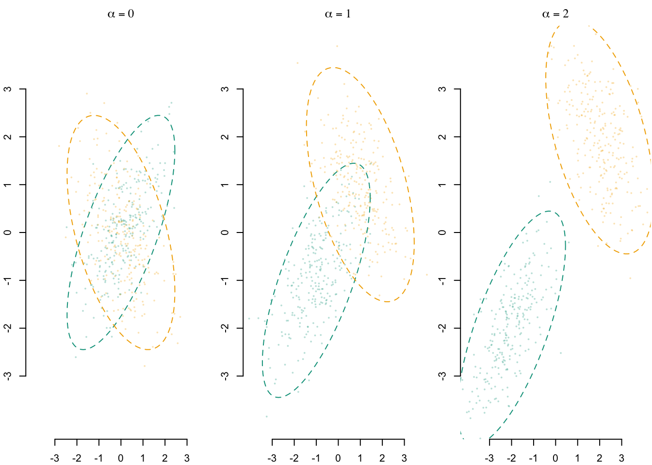
A visual representation of the samples that can be drawn from the DGP with three values of \(\alpha\) is provided in Figure 6.1.
Codes to create the Figure.
library(tikzDevice)
export_tikz <- FALSE

scale <- 1.7

if (export_tikz == TRUE) {
  filename <- "gaussian-example-alpha"
  tikz(paste0("figs/", filename, ".tex"), width = scale*2.2, height = scale*1)
}

draw_ellipse <- function(mu,
                         sigma,
                         col = "black",
                         lty = 1,
                         lwd = 1,
                         level = 0.95,
                         ...) {

  angles <- seq(0, 2 * pi, length.out = 100)
  vals <- sqrt(
    qchisq(level, df = 2)) * t(chol(sigma)) %*% rbind(cos(angles), sin(angles)
    )
  lines(mu[1] + vals[1, ], mu[2] + vals[2, ], col = col, lty = lty, lwd = lwd, ...)

}

set.seed(123)

mu0 <- -1
mu1 <- +1
r0 <- +.7
r1 <- -.5

# Generate data with alpha=0, alpha=1, alpha=2
data_alpha_0 <- gen_data(a = 0, mu0 = mu0, mu1 = mu1, r0 = r0, r1 = r1)
data_alpha_1 <- gen_data(a = 1, mu0 = mu0, mu1 = mu1, r0 = r0, r1 = r1)
data_alpha_2 <- gen_data(a = 2, mu0 = mu0, mu1 = mu1, r0 = r0, r1 = r1)


par(mar = c(2.1, 2.1, 2.1, 0.1), mfrow = c(1, 3))
x_lim <- c(-4, 4)
y_lim <- c(-4, 4)
cex_pts <- .4

# With alpha=0----
a <- 0

x_lab <- "$\\alpha = 0$"
if (export_tikz == FALSE) x_lab <- latex2exp::TeX(x_lab)

plot(
  data_alpha_0$X1[data_alpha_0$A == 0],
  data_alpha_0$X2[data_alpha_0$A == 0],
  pch = 16,
  cex = cex_pts,
  col = adjustcolor(colGpe0, alpha = .3),
  xlim = x_lim, ylim = y_lim,
  xlab = "", ylab = "",
  main = x_lab,
  family = font_family,
  axes = FALSE
)
axis(1, at = -3:3)
axis(2, at = -3:3)
title(xlab = "X1", ylab="X2", line=2, cex.lab=1.2, family = font_family)
points(
  data_alpha_0$X1[data_alpha_0$A == 1],
  data_alpha_0$X2[data_alpha_0$A == 1],
  col = adjustcolor(colGpe1, alpha = .3), pch = 16, cex = cex_pts
)

# True mean and covariance (scaled by 'a')
Mu0 <- rep(a * mu0, 2)
Mu1 <- rep(a * mu1, 2)
Sig0 <- matrix(c(1, r0, r0, 1), 2, 2)
Sig1 <- matrix(c(1, r1, r1, 1), 2, 2)


# Add ellipses
draw_ellipse(Mu0, Sig0, col = colGpe0, lty = 2)
draw_ellipse(Mu1, Sig1, col = colGpe1, lty = 2)

# With alpha=1----
a <- 1

x_lab <- "$\\alpha = 1$"
if (export_tikz == FALSE) x_lab <- latex2exp::TeX(x_lab)

plot(
  data_alpha_1$X1[data_alpha_1$A == 0],
  data_alpha_1$X2[data_alpha_1$A == 0],
  pch = 16, cex = cex_pts,
  col = adjustcolor(colGpe0, alpha = .3),
  xlim = x_lim, ylim = y_lim,
  xlab = "", ylab = "",
  main = x_lab,
  family = font_family,
  axes = FALSE
)
axis(1, at = -3:3)
axis(2, at = -3:3)
title(xlab = "X1", ylab="X2", line=2, cex.lab=1.2, family = font_family)
points(
  data_alpha_1$X1[data_alpha_1$A == 1],
  data_alpha_1$X2[data_alpha_1$A == 1],
  col = adjustcolor(colGpe1, alpha = .3), pch = 16, cex = cex_pts
)

# True mean and covariance (scaled by 'a')
Mu0 <- rep(a * mu0, 2)
Mu1 <- rep(a * mu1, 2)
Sig0 <- matrix(c(1, r0, r0, 1), 2, 2)
Sig1 <- matrix(c(1, r1, r1, 1), 2, 2)

# Add ellipses
draw_ellipse(Mu0, Sig0, col = colGpe0, lty = 2)
draw_ellipse(Mu1, Sig1, col = colGpe1, lty = 2)

# With alpha=2----
a <- 2

x_lab <- "$\\alpha = 2$"
if (export_tikz == FALSE) x_lab <- latex2exp::TeX(x_lab)

plot(
  data_alpha_2$X1[data_alpha_2$A == 0],
  data_alpha_2$X2[data_alpha_2$A == 0],
  pch = 16, cex = cex_pts,
  col = adjustcolor(colGpe0, alpha = .3),
  xlim = x_lim, ylim = y_lim,
  xlab = "", ylab = "",
  main = x_lab,
  family = font_family,
  axes = FALSE
)
axis(1, at = -3:3)
axis(2, at = -3:3)
title(xlab = "X1", ylab="X2", line=2, cex.lab=1.2, family = font_family)
points(
  data_alpha_2$X1[data_alpha_2$A == 1],
  data_alpha_2$X2[data_alpha_2$A == 1],
  col = adjustcolor(colGpe1, alpha = .3), pch = 16, cex = cex_pts
)

# True mean and covariance (scaled by 'a')
Mu0 <- rep(a * mu0, 2)
Mu1 <- rep(a * mu1, 2)
Sig0 <- matrix(c(1, r0, r0, 1), 2, 2)
Sig1 <- matrix(c(1, r1, r1, 1), 2, 2)

# Add ellipses
draw_ellipse(Mu0, Sig0, col = colGpe0, lty = 2)
draw_ellipse(Mu1, Sig1, col = colGpe1, lty = 2)

if (export_tikz == TRUE) {
  dev.off()
  plot_to_pdf(
    filename = filename, path = "./figs/", keep_tex = FALSE, crop = FALSE
  )
}
We define a grid with the different simulations.
n_repl <- 200
grid_params <- expand_grid(
  n0 = 250,
  n1 = 250,
  mu0 = -1,
  mu1 = +1,
  r0 = +.7,
  r1 = -.5,
  a = seq(0, 2, by = .1),
  seed = seq_len(n_repl)
)
The simulations can be run in parallel.
The codes to run the simulations
# This chunk takes about XX minutes to run.
# We do not evaluate when compiling the document.
# Instead, we load previously obtained results.
library(pbapply)
library(parallel)
ncl <- detectCores()-1
(cl <- makeCluster(ncl))

clusterEvalQ(cl, {
  library(tidyverse)
  library(mnormt)
  library(expm)
  library(randomForest)
  library(fairadapt)
}) |>
  invisible()

clusterExport(
  cl = cl, c(
    "gen_data", "compute_ot_map", "apply_ot_transport",
    "transport_regul", "transport_many_to_one",
    "sequential_transport_12", "sequential_transport_21",
    "causal_effects_cf", "sim_f", "grid_params", "fairadapt_12",
    "fairadapt_21"
  )
)

# For an unknown reason, there seems to be an issue with performing this in
# one go. Let us divide the task into two.

res_sim_1 <- pbapply::pblapply(1:2100, function(i) {

  grid_params_current <- grid_params[i, ]

  n0 <- grid_params_current$n0
  n1 <- grid_params_current$n1
  mu0 <- grid_params_current$mu0
  mu1 <- grid_params_current$mu1
  r0 <- grid_params_current$r0
  r1 <- grid_params_current$r1
  a <- grid_params_current$a
  seed <- grid_params_current$seed

  sim_f(
    n0 = n0, n1 = n1,
    mu0 = mu0, mu1 = mu1,
    r0 = r0, r1 = r1,
    a = a, seed = seed
  )
}, cl = cl)

res_sim_2 <- pbapply::pblapply(2101:nrow(grid_params), function(i) {

  grid_params_current <- grid_params[i, ]

  n0 <- grid_params_current$n0
  n1 <- grid_params_current$n1
  mu0 <- grid_params_current$mu0
  mu1 <- grid_params_current$mu1
  r0 <- grid_params_current$r0
  r1 <- grid_params_current$r1
  a <- grid_params_current$a
  seed <- grid_params_current$seed

  sim_f(
    n0 = n0, n1 = n1,
    mu0 = mu0, mu1 = mu1,
    r0 = r0, r1 = r1,
    a = a, seed = seed
  )
}, cl = cl)

res_sim_1 <- list_rbind(res_sim_1)
res_sim_2 <- list_rbind(res_sim_2)

res_sim <- res_sim_1 |> bind_rows(res_sim_2)

stopCluster(cl)


save(res_sim, file = "../output/res_sim-gaussian-mc.rda")
We load previously obtained results:
load("../output/res_sim-gaussian-mc.rda")Codes to create the Figure.
a1 <- 2
a2 <- -1.5
export_pdf <- FALSE

x_lab <- "$\\alpha$ (distance $=2\\alpha\\sqrt{2}$)"
y_lab <- "Distance to $\\bar\\tau$"

if (export_pdf == FALSE) {
  x_lab <- latex2exp::TeX(x_lab)
  y_lab <- latex2exp::TeX(y_lab)
}

data_plot <- res_sim |>
  dplyr::select(
    n0, n1, seed, a, mu0, mu1,
    tot_effect_med, tot_effect_ot, tot_effect_tmatch,
    tot_effect_skh, tot_effect_sot_12, tot_effect_sot_21,
    tot_effect_fairadapt_12_lin, tot_effect_fairadapt_21_lin
  ) |>
  pivot_longer(
    cols = c(
      tot_effect_med, tot_effect_ot, tot_effect_tmatch,
      tot_effect_skh, tot_effect_sot_12, tot_effect_sot_21,
      tot_effect_fairadapt_12_lin, tot_effect_fairadapt_21_lin
    ),
    names_to = "type", values_to = "tau"
  ) |>
  mutate(
    type = factor(
      type,
      levels = c(
        "tot_effect_med", "tot_effect_ot", "tot_effect_tmatch",
        "tot_effect_skh", "tot_effect_sot_12", "tot_effect_sot_21",
        "tot_effect_fairadapt_12_lin", "tot_effect_fairadapt_21_lin"
      ),
      labels = c("CM", "OT", "OT-M", "SKH", "ST(1)", "ST(2)", "FPT(1)", "FPT(2)")
    ),
    dist_to_causal_effect = (a1+a2) * (a*mu1 - a*mu0) + 3 - tau
  )

p <- ggplot(
  data = data_plot,
  mapping = aes(x = factor(a), y = dist_to_causal_effect)
) +
  geom_violin(
    mapping = aes(fill = type)
  ) +
  geom_hline(yintercept = 0, colour = "darkred", linetype = "dashed") +
  theme_paper() +
  facet_wrap(~type, scales = "free_x", ncol = 2) +
  scale_fill_manual(
    NULL,
    values = c(
      "CM" = "#56B4E9",
      "OT" = colour_methods[["OT"]],
      "OT-M" = colour_methods[["OT-M"]],
      "SKH" = colour_methods[["skh"]],
      "ST(1)" =  colour_methods[["seq_1"]],
      "ST(2)" =  colour_methods[["seq_2"]],
      "FPT(1)" =  colour_methods[["fairadapt_1"]],
      "FPT(2)" =  colour_methods[["fairadapt_2"]]
    ),
    guide = "none",
  ) +
  theme(legend.position = "bottom") +
  labs(
    x = x_lab,
    y = y_lab,
  ) +
  scale_x_discrete(
    labels = ifelse(unique(data_plot$a) %% .5 == 0, unique(data_plot$a), "")
  )

if (export_pdf == TRUE) {
  filename <- "gaussian-mc-alpha-tau"
  ggplot2_to_pdf(
    plot = p + theme(panel.spacing = unit(0.4, "lines")),
    filename = filename, path = "figs/",
    width = 3.3, height = 3.5,
    crop = TRUE
  )

  system(paste0("pdfcrop figs/", filename, ".pdf figs/", filename, ".pdf"))
}

p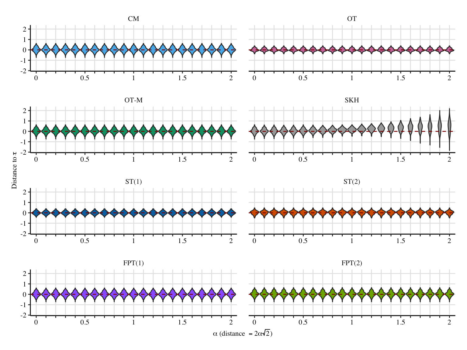
Codes to create the Figure.
export_pdf <- FALSE

x_lab <- "$\\alpha$ (distance $=2\\alpha\\sqrt{2}$)"
# y_lab <- "Distance to $\\bar\\delta(0)$"
y_lab <- "Distance to $\\bar\\delta$"

if (export_pdf == FALSE) {
  x_lab <- latex2exp::TeX(x_lab)
  y_lab <- latex2exp::TeX(y_lab)
}

data_plot <- res_sim |>
  dplyr::select(
    n0, n1, seed, a, mu0, mu1,
    delta_0_med, delta_0_ot, delta_0_tmatch,
    delta_0_skh, delta_0_sot_12, delta_0_sot_21,
    delta_0_fairadapt_12_lin, delta_0_fairadapt_21_lin
  ) |>
  pivot_longer(
    cols = c(
      delta_0_med, delta_0_ot, delta_0_tmatch,
      delta_0_skh, delta_0_sot_12, delta_0_sot_21,
      delta_0_fairadapt_12_lin, delta_0_fairadapt_21_lin
    ),
    names_to = "type", values_to = "val"
  ) |>
  mutate(
    type = factor(
      type,
      levels = c(
        "delta_0_med", "delta_0_ot", "delta_0_tmatch",
        "delta_0_skh", "delta_0_sot_12", "delta_0_sot_21",
        "delta_0_fairadapt_12_lin", "delta_0_fairadapt_21_lin"
      ),
      labels = c("CM", "OT", "OT-M", "SKH", "ST(1)", "ST(2)", "FPT(1)", "FPT(2)")
    ),
    dist_to_theo_val = ((a1+a2)*(a*mu1-a*mu0)) - val
  )

p <- ggplot(
  data = data_plot,
  mapping = aes(x = factor(a), y = dist_to_theo_val)
) +
  geom_violin(
    mapping = aes(fill = type)
  ) +
  geom_hline(yintercept = 0, colour = "darkred", linetype = "dashed") +
  theme_paper() +
  facet_wrap(~type, scales = "free_x", ncol = 2) +
  scale_fill_manual(
    NULL,
    values = c(
      "CM" = "#56B4E9",
      "OT" = colour_methods[["OT"]],
      "OT-M" = colour_methods[["OT-M"]],
      "SKH" = colour_methods[["skh"]],
      "ST(1)" =  colour_methods[["seq_1"]],
      "ST(2)" =  colour_methods[["seq_2"]],
      "FPT(1)" =  colour_methods[["fairadapt_1"]],
      "FPT(2)" =  colour_methods[["fairadapt_2"]]
    ),
    guide = "none"
  ) +
  theme(legend.position = "bottom") +
  labs(
    x = x_lab,
    y = y_lab,
  ) +
  scale_x_discrete(
    labels = ifelse(unique(data_plot$a) %% .5 == 0, unique(data_plot$a), "")
  )

if (export_pdf == TRUE) {
  filename <- "gaussian-mc-alpha-delta0"
  ggplot2_to_pdf(
    plot = p + theme(panel.spacing = unit(0.4, "lines")),
    filename = filename, path = "figs/",
    width = 3.3, height = 3.5,
    crop = TRUE
  )

  system(paste0("pdfcrop figs/", filename, ".pdf figs/", filename, ".pdf"))
}
p
Codes to create the Figure.
data_plot <- res_sim |>
  dplyr::select(
    n0, n1, seed, a, mu0, mu1,
    delta_1_med, delta_1_ot, delta_1_tmatch,
    delta_1_skh, delta_1_sot_12, delta_1_sot_21,
    delta_1_fairadapt_12_lin, delta_1_fairadapt_21_lin
  ) |>
  pivot_longer(
    cols = c(
    delta_1_med, delta_1_ot, delta_1_tmatch,
    delta_1_skh, delta_1_sot_12, delta_1_sot_21,
    delta_1_fairadapt_12_lin, delta_1_fairadapt_21_lin),
    names_to = "type", values_to = "val"
  ) |>
  mutate(
    type = factor(
      type,
      levels = c(
        "delta_1_med", "delta_1_ot", "delta_1_tmatch",
        "delta_1_skh", "delta_1_sot_12", "delta_1_sot_21",
        "delta_1_fairadapt_12_lin", "delta_1_fairadapt_21_lin"
      ),
      labels = c("CM", "OT", "OT-M", "SKH", "ST(1)", "ST(2)", "FPT(1)", "FPT(2)")
    ),
    dist_to_theo_val = ((a1+a2)*(a*mu1-a*mu0)) - val
  )
ggplot(
  data = data_plot,
  mapping = aes(x = factor(a), y = dist_to_theo_val)
) +
  geom_violin(
    mapping = aes(fill = type)
  ) +
  geom_hline(yintercept = 0, colour = "darkred", linetype = "dashed") +
  theme_paper() +
  facet_wrap(~type, scales = "free_x", ncol = 2) +
  scale_fill_manual(
    NULL,
    values = c(
      "CM" = "#56B4E9",
      "OT" = colour_methods[["OT"]],
      "OT-M" = colour_methods[["OT-M"]],
      "SKH" = colour_methods[["skh"]],
      "ST(1)" =  colour_methods[["seq_1"]],
      "ST(2)" =  colour_methods[["seq_2"]],
      "FPT(1)" =  colour_methods[["fairadapt_1"]],
      "FPT(2)" =  colour_methods[["fairadapt_2"]]
    ),
    guide = "none"
  ) +
  theme(legend.position = "bottom") +
  labs(
    x = latex2exp::TeX("$\\alpha$ (distance $=2\\alpha\\sqrt{2}$)"),
    y = "Distance to theoretical natural indirect effect",
  ) +
  scale_x_discrete(
    labels = ifelse(unique(data_plot$a) %% .5 == 0, unique(data_plot$a), "")
  )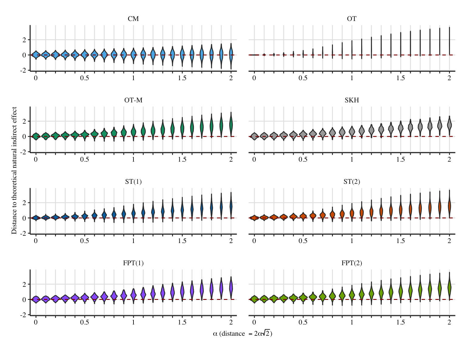
Codes to create the Figure.
data_plot <- res_sim |>
dplyr::select(
n0, n1, seed, a, mu0, mu1,
zeta_0_med, zeta_0_ot, zeta_0_tmatch,
zeta_0_skh, zeta_0_sot_12, zeta_0_sot_21,
zeta_0_fairadapt_12_lin, zeta_0_fairadapt_21_lin
) |>
pivot_longer(
cols = c(zeta_0_med, zeta_0_ot, zeta_0_tmatch,
zeta_0_skh, zeta_0_sot_12, zeta_0_sot_21,
zeta_0_fairadapt_12_lin, zeta_0_fairadapt_21_lin),
names_to = "type", values_to = "val"
) |>
mutate(
type = factor(
type,
levels = c(
"zeta_0_med", "zeta_0_ot", "zeta_0_tmatch",
"zeta_0_skh", "zeta_0_sot_12", "zeta_0_sot_21",
"zeta_0_fairadapt_12_lin", "zeta_0_fairadapt_21_lin"
),
labels = c("CM", "OT", "OT-M", "SKH", "ST(1)", "ST(2)", "FPT(1)", "FPT(2)")
),
dist_to_theo_val = 3 - val
)
ggplot(
data = data_plot,
mapping = aes(x = factor(a), y = dist_to_theo_val)
) +
geom_violin(
mapping = aes(fill = type)
) +
geom_hline(yintercept = 0, colour = "darkred", linetype = "dashed") +
theme_paper() +
facet_wrap(~type, scales = "free_x", ncol = 2) +
scale_fill_manual(
NULL,
values = c(
"CM" = "#56B4E9",
"OT" = colour_methods[["OT"]],
"OT-M" = colour_methods[["OT-M"]],
"SKH" = colour_methods[["skh"]],
"ST(1)" = colour_methods[["seq_1"]],
"ST(2)" = colour_methods[["seq_2"]],
"FPT(1)" = colour_methods[["fairadapt_1"]],
"FPT(2)" = colour_methods[["fairadapt_2"]]
),
guide = "none"
) +
theme(legend.position = "bottom") +
labs(
x = latex2exp::TeX("$\\alpha$ (distance $=2\\alpha\\sqrt{2}$)"),
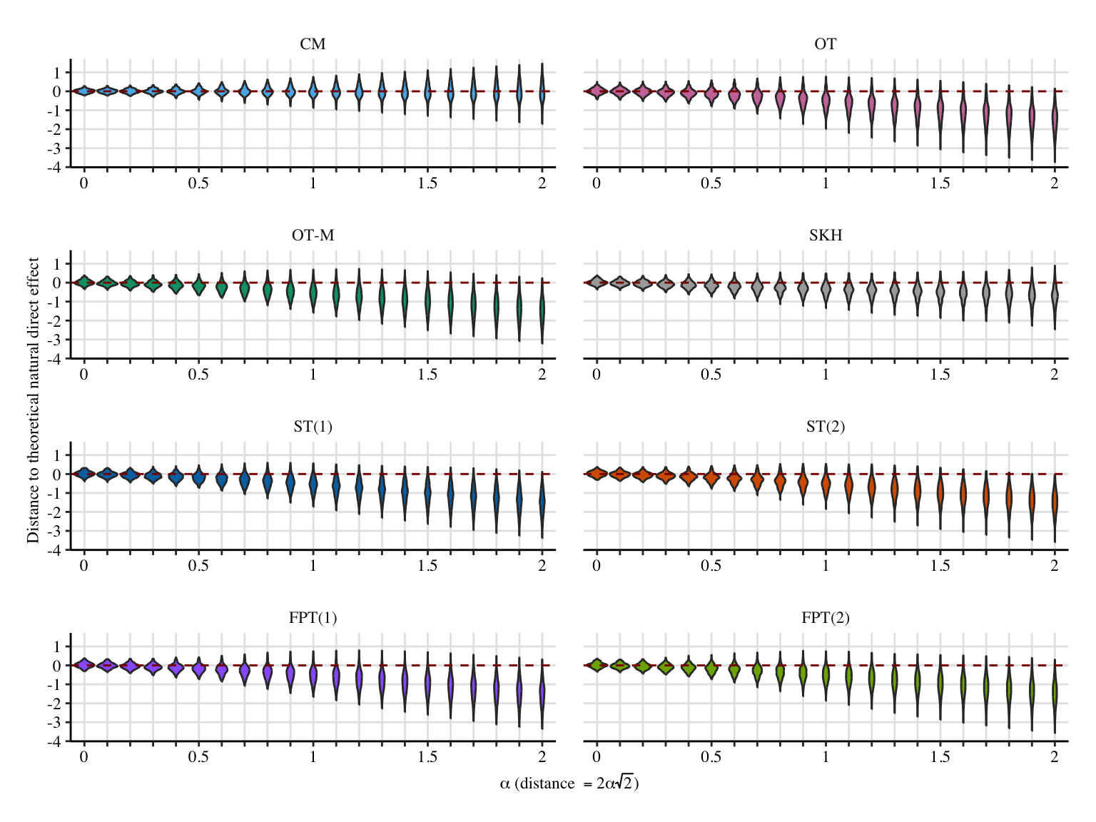
y = "Distance to theoretical natural direct effect",
) +
scale_x_discrete(
labels = ifelse(unique(data_plot$a) %% .5 == 0, unique(data_plot$a), "")
)
Codes to create the Figure.
p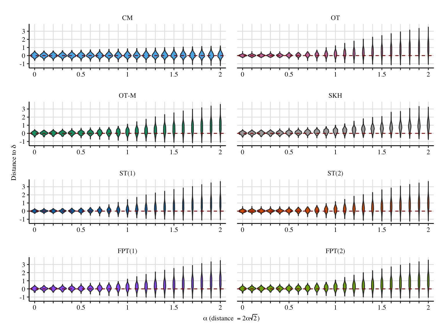
Codes to create the Figure.
export_pdf <- FALSE

x_lab <- "$\\alpha$ (distance $=2\\alpha\\sqrt{2}$)"
# y_lab <- "Distance to $\\bar\\zeta(1)$"
y_lab <- "Distance to $\\bar\\zeta$"

if (export_pdf == FALSE) {
  x_lab <- latex2exp::TeX(x_lab)
  y_lab <- latex2exp::TeX(y_lab)
}

data_plot <- res_sim |>
  dplyr::select(
    n0, n1, seed, a, mu0, mu1,
    zeta_1_med, zeta_1_ot, zeta_1_tmatch,
    zeta_1_skh, zeta_1_sot_12, zeta_1_sot_21,
    zeta_1_fairadapt_12_lin, zeta_1_fairadapt_21_lin
  ) |>
  pivot_longer(
    cols = c(
      zeta_1_med, zeta_1_ot, zeta_1_tmatch,
      zeta_1_skh, zeta_1_sot_12, zeta_1_sot_21,
      zeta_1_fairadapt_12_lin, zeta_1_fairadapt_21_lin),
    names_to = "type", values_to = "val"
  ) |>
  mutate(
    type = factor(
      type,
      levels = c(
        "zeta_1_med", "zeta_1_ot", "zeta_1_tmatch",
        "zeta_1_skh", "zeta_1_sot_12", "zeta_1_sot_21",
        "zeta_1_fairadapt_12_lin", "zeta_1_fairadapt_21_lin"
      ),
      labels = c("CM", "OT", "OT-M", "SKH", "ST(1)", "ST(2)", "FPT(1)", "FPT(2)")
    ),
    dist_to_theo_val = 3 - val
  )
p <- ggplot(
  data = data_plot,
  mapping = aes(x = factor(a), y = dist_to_theo_val)
) +
  geom_violin(
    mapping = aes(fill = type)
  ) +
  geom_hline(yintercept = 0, colour = "darkred", linetype = "dashed") +
  theme_paper() +
  facet_wrap(~type, scales = "free_x", ncol = 2) +
  scale_fill_manual(
    NULL,
    values = c(
      "CM" = "#56B4E9",
      "OT" = colour_methods[["OT"]],
      "OT-M" = colour_methods[["OT-M"]],
      "SKH" = colour_methods[["skh"]],
      "ST(1)" =  colour_methods[["seq_1"]],
      "ST(2)" =  colour_methods[["seq_2"]],
      "FPT(1)" =  colour_methods[["fairadapt_1"]],
      "FPT(2)" =  colour_methods[["fairadapt_2"]]
    ),
    guide = "none"
  ) +
  theme(legend.position = "bottom") +
  labs(
    x = x_lab,
    y = y_lab,
  ) +
  scale_x_discrete(
    labels = ifelse(unique(data_plot$a) %% .5 == 0, unique(data_plot$a), "")
  )

if (export_pdf == TRUE) {
  filename <- "gaussian-mc-alpha-zeta1"
  ggplot2_to_pdf(
    plot = p + theme(panel.spacing = unit(0.4, "lines")),
    filename = filename, path = "figs/",
    width = 3.3, height = 3.5,
    crop = TRUE
  )

  system(paste0("pdfcrop figs/", filename, ".pdf figs/", filename, ".pdf"))
}

p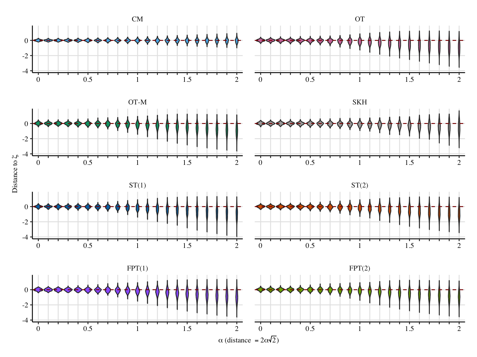
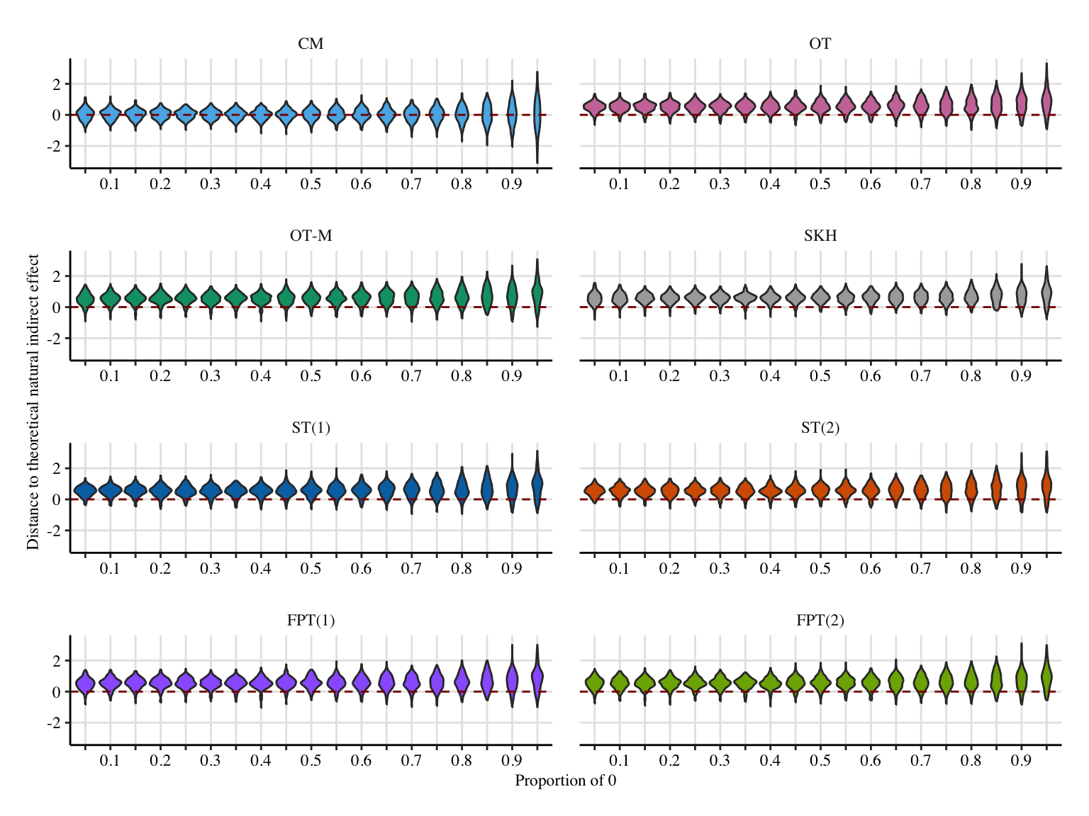
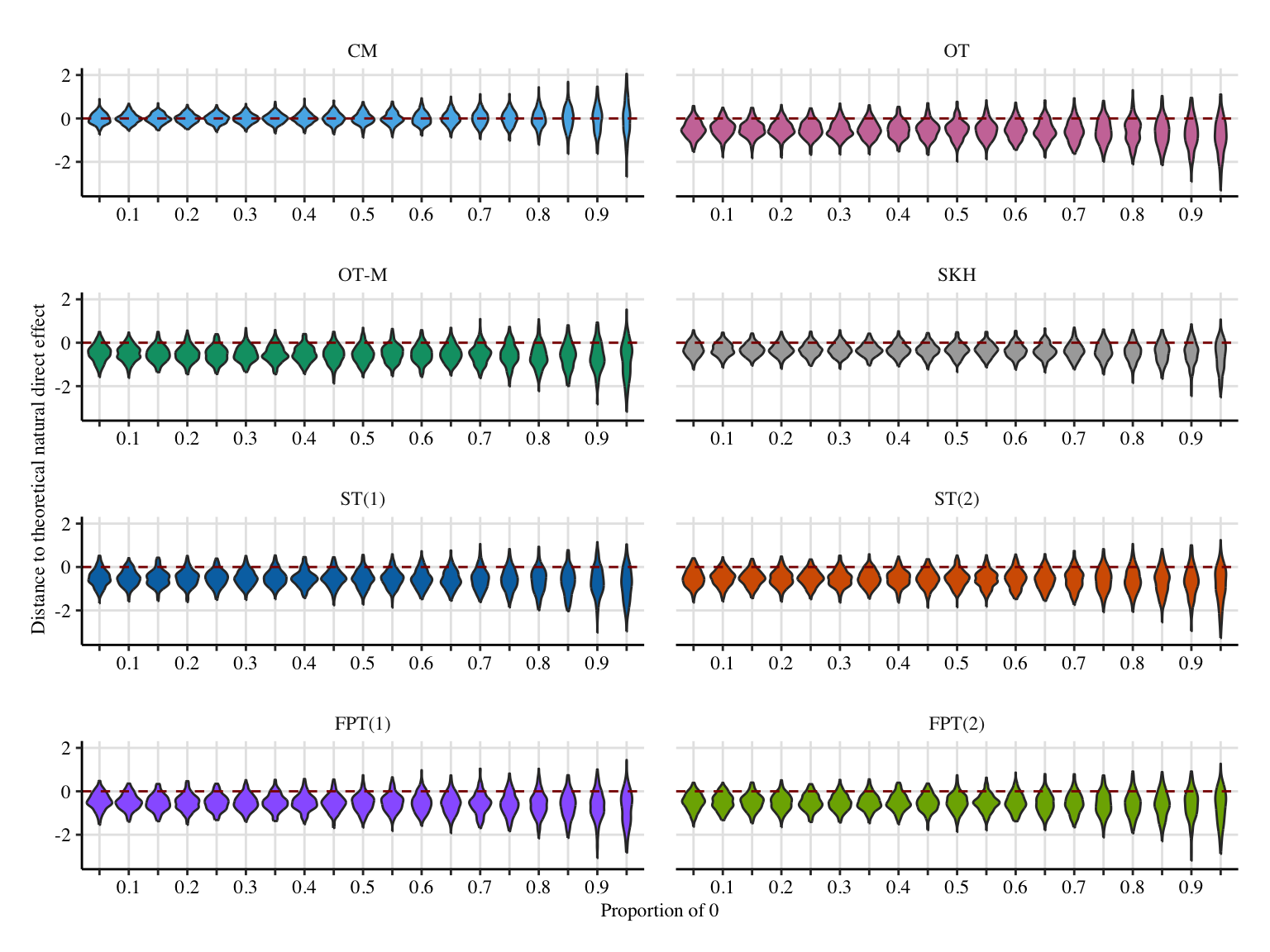
A more condensed figure, which focuses on \(\bar{\delta}(0)\), \(\bar{\zeta}(1)\), and \(\bar{\tau}\).
Codes to create the Figure.
a1 <- 2
a2 <- -1.5


x_lab <- "$\\alpha$ (distance $=2\\alpha\\sqrt{2}$)"
y_lab <- "Estimation error"
metrics_lab <- c("$\\bar{\\delta}(0)$", "$\\bar{\\zeta}(1)$", "$\\bar{\\tau}$")
metrics_lab <- c("$\\bar{\\delta}$", "$\\bar{\\zeta}$", "$\\bar{\\tau}$")


x_lab <- latex2exp::TeX(x_lab)
y_lab <- latex2exp::TeX(y_lab)
metrics_lab <- latex2exp::TeX(metrics_lab)


data_plot_tau <- res_sim |>
  dplyr::select(
    n0, n1, seed, a, mu0, mu1,
    tot_effect_med,
    tot_effect_fairadapt_12_lin, tot_effect_fairadapt_21_lin,
    tot_effect_ot, tot_effect_tmatch,
    tot_effect_skh, tot_effect_sot_12, tot_effect_sot_21
  ) |>
  pivot_longer(
    cols = c(
      tot_effect_med,
      tot_effect_fairadapt_12_lin, tot_effect_fairadapt_21_lin,
      tot_effect_ot, tot_effect_tmatch,
      tot_effect_skh, tot_effect_sot_12, tot_effect_sot_21
    ),
    names_to = "type", values_to = "tau"
  ) |>
  mutate(
    type = factor(
      type,
      levels = c(
        "tot_effect_med",
        "tot_effect_fairadapt_12_lin", "tot_effect_fairadapt_21_lin",
        "tot_effect_ot", "tot_effect_tmatch",
        "tot_effect_skh", "tot_effect_sot_12", "tot_effect_sot_21"
      ),
      labels = c("CM", "FPT(1)", "FPT(2)", "OT", "OT-M", "SKH", "ST(1)", "ST(2)")
    ),
    dist_to_causal_effect = (a1+a2) * (a*mu1 - a*mu0) + 3 - tau
  )

data_plot_delta0 <- res_sim |>
  dplyr::select(
    n0, n1, seed, a, mu0, mu1,
    delta_0_med,
    delta_0_fairadapt_12_lin, delta_0_fairadapt_21_lin,
    delta_0_ot, delta_0_tmatch,
    delta_0_skh, delta_0_sot_12, delta_0_sot_21
  ) |>
  pivot_longer(
    cols = c(
      delta_0_med,
      delta_0_fairadapt_12_lin, delta_0_fairadapt_21_lin,
      delta_0_ot, delta_0_tmatch,
      delta_0_skh, delta_0_sot_12, delta_0_sot_21
    ),
    names_to = "type", values_to = "val"
  ) |>
  mutate(
    type = factor(
      type,
      levels = c(
        "delta_0_med",
        "delta_0_fairadapt_12_lin", "delta_0_fairadapt_21_lin",
        "delta_0_ot", "delta_0_tmatch",
        "delta_0_skh", "delta_0_sot_12", "delta_0_sot_21"
      ),
      labels = c("CM", "FPT(1)", "FPT(2)", "OT", "OT-M", "SKH", "ST(1)", "ST(2)")
    ),
    dist_to_theo_val = ((a1+a2)*(a*mu1-a*mu0)) - val
  )

data_plot_zeta1 <- res_sim |>
  dplyr::select(
    n0, n1, seed, a, mu0, mu1,
    zeta_1_med,
    zeta_1_fairadapt_12_lin, zeta_1_fairadapt_21_lin,
    zeta_1_ot, zeta_1_tmatch,
    zeta_1_skh, zeta_1_sot_12, zeta_1_sot_21
  ) |>
  pivot_longer(
    cols = c(
      zeta_1_med, zeta_1_ot, zeta_1_tmatch,
      zeta_1_fairadapt_12_lin, zeta_1_fairadapt_21_lin,
      zeta_1_skh, zeta_1_sot_12, zeta_1_sot_21),
    names_to = "type", values_to = "val"
  ) |>
  mutate(
    type = factor(
      type,
      levels = c(
        "zeta_1_med",
        "zeta_1_fairadapt_12_lin", "zeta_1_fairadapt_21_lin",
        "zeta_1_ot", "zeta_1_tmatch",
        "zeta_1_skh", "zeta_1_sot_12", "zeta_1_sot_21"
      ),
      labels = c("CM", "FPT(1)", "FPT(2)", "OT", "OT-M", "SKH", "ST(1)", "ST(2)")
    ),
    dist_to_theo_val = 3 - val
  )

data_plot <- data_plot_tau |>
  rename(dist_tau = dist_to_causal_effect) |>
  left_join(
    data_plot_delta0 |>
      rename(
        delta0 = val,
        dist_delta0 = dist_to_theo_val
      ),
    by = c("n0", "n1", "seed", "a", "mu0", "mu1", "type")
  ) |>
  left_join(
    data_plot_zeta1 |>
      rename(
        zeta1 = val,
        dist_zeta1 = dist_to_theo_val
      ),
    by = c("n0", "n1", "seed", "a", "mu0", "mu1", "type")
  ) |>
filter(a %in% seq(0, 2, by = .2))

p <- ggplot(
  data = data_plot |> select(-tau, -delta0, -zeta1) |>
    pivot_longer(
      cols = c(dist_tau, dist_delta0, dist_zeta1),
      names_to = "metric",
      values_to = "dist"
    ) |>
    mutate(
      metric = factor(
        metric,
        levels = c("dist_delta0", "dist_zeta1", "dist_tau"),
        labels = metrics_lab
      )
    ),
  mapping = aes(x = factor(a), y = dist)
) +
  geom_violin(
    mapping = aes(fill = type)
  ) +
  geom_hline(yintercept = 0, colour = "darkred", linetype = "dashed") +
  theme_paper() +
  facet_grid(metric ~ type, scales = "free_x") +
  scale_fill_manual(
    NULL,
    values = c(
      "CM" = "#56B4E9",
      "FPT(1)" =  colour_methods[["fairadapt_1"]],
      "FPT(2)" =  colour_methods[["fairadapt_2"]],
      "OT" = colour_methods[["OT"]],
      "OT-M" = colour_methods[["OT-M"]],
      "SKH" = colour_methods[["skh"]],
      "ST(1)" =  colour_methods[["seq_1"]],
      "ST(2)" =  colour_methods[["seq_2"]]
    ),
    guide = "none",
  ) +
  theme(legend.position = "bottom") +
  labs(
    x = x_lab,
    y = y_lab,
  ) +
  scale_x_discrete(
    labels = ifelse(unique(data_plot$a) %% .5 == 0, unique(data_plot$a), "")
  )

p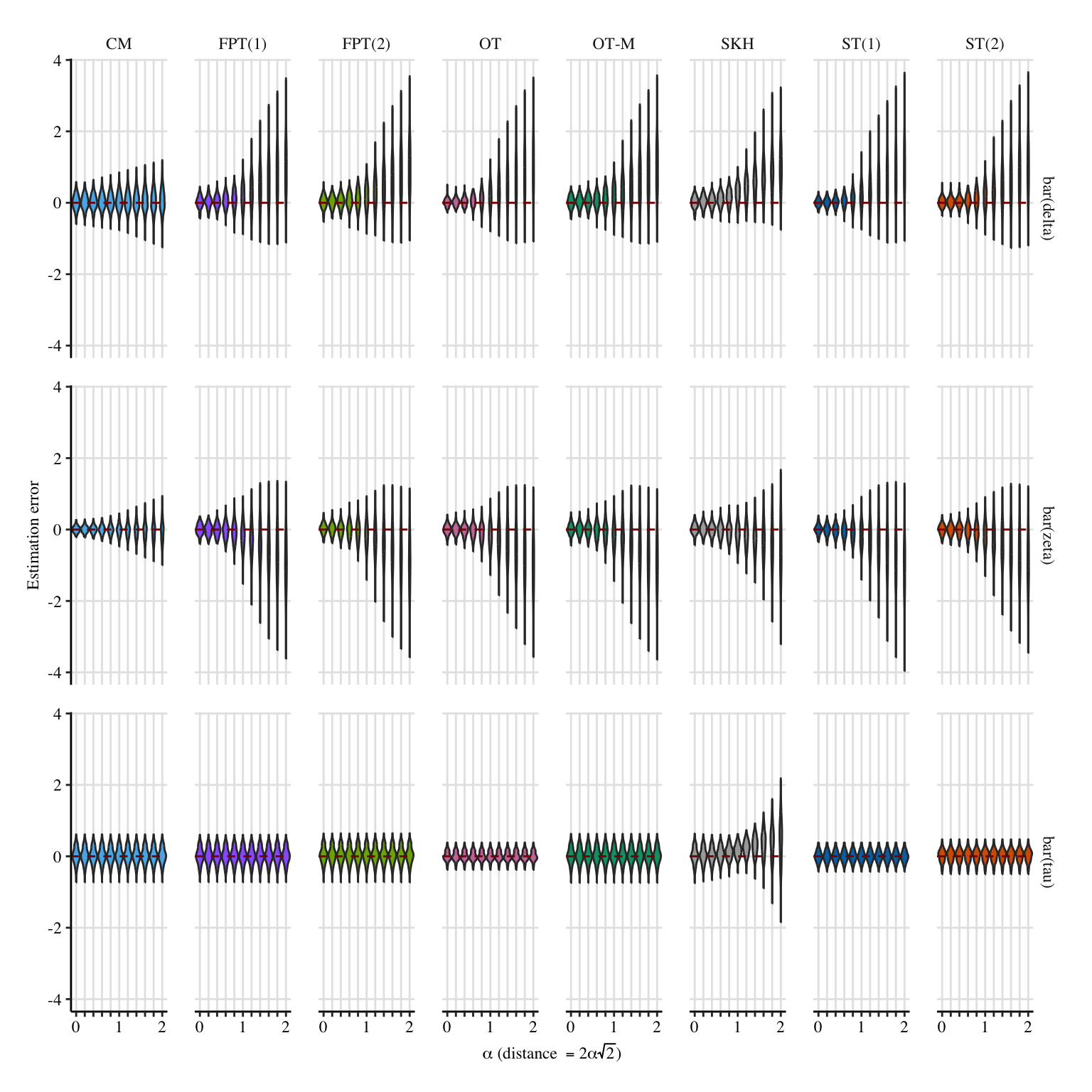
A shorter version for the paper.
Codes to create the Figure.
a1 <- 2
a2 <- -1.5
export_pdf <- TRUE #FALSE

x_lab <- "$\\alpha$ (distance $=2\\alpha\\sqrt{2}$)"
y_lab <- "Estimation error"
metrics_lab <- c("$\\bar{\\delta}(0)$", "$\\bar{\\zeta}(1)$", "$\\bar{\\tau}$")
metrics_lab <- c("$\\bar{\\delta}$", "$\\bar{\\zeta}$", "$\\bar{\\tau}$")

if (export_pdf == FALSE) {
  x_lab <- latex2exp::TeX(x_lab)
  y_lab <- latex2exp::TeX(y_lab)
  metrics_lab <- latex2exp::TeX(metrics_lab)
}

data_plot <- data_plot_tau |>
  rename(dist_tau = dist_to_causal_effect) |>
  left_join(
    data_plot_delta0 |>
      rename(
        delta0 = val,
        dist_delta0 = dist_to_theo_val
      ),
    by = c("n0", "n1", "seed", "a", "mu0", "mu1", "type")
  ) |>
  left_join(
    data_plot_zeta1 |>
      rename(
        zeta1 = val,
        dist_zeta1 = dist_to_theo_val
      ),
    by = c("n0", "n1", "seed", "a", "mu0", "mu1", "type")
  ) |>
  filter(a %in% seq(0, 2, by = .2)) |>
  filter(type %in% c("ST(1)", "ST(2)", "OT", "SKH", "OT"))


p <- ggplot(
  data = data_plot |> select(-tau, -delta0, -zeta1) |>
    pivot_longer(
      cols = c(dist_tau, dist_delta0, dist_zeta1),
      names_to = "metric",
      values_to = "dist"
    ) |>
    mutate(
      metric = factor(
        metric,
        levels = c("dist_delta0", "dist_zeta1", "dist_tau"),
        labels = metrics_lab
      )
    ),
  mapping = aes(x = factor(a), y = dist)
) +
  geom_violin(
    mapping = aes(fill = type)
  ) +
  geom_hline(yintercept = 0, colour = "darkred", linetype = "dashed") +
  theme_paper() +
  facet_grid(metric ~ type, scales = "free_x") +
  scale_fill_manual(
    NULL,
    values = c(
      "CM" = "#56B4E9",
      "FPT(1)" =  colour_methods[["fairadapt_1"]],
      "FPT(2)" =  colour_methods[["fairadapt_2"]],
      "OT" = colour_methods[["OT"]],
      "OT-M" = colour_methods[["OT-M"]],
      "SKH" = colour_methods[["skh"]],
      "ST(1)" =  colour_methods[["seq_1"]],
      "ST(2)" =  colour_methods[["seq_2"]]
    ),
    guide = "none",
  ) +
  theme(legend.position = "bottom") +
  labs(
    x = x_lab,
    y = y_lab,
  ) +
  scale_x_discrete(
    labels = ifelse(unique(data_plot$a) %% .5 == 0, unique(data_plot$a), "")
  )

scale <- .77
if (export_pdf == TRUE) {
  filename <- "gaussian-mc-alpha"
  ggplot2_to_pdf(
    plot = p + theme(panel.spacing = unit(0.4, "lines")),
    filename = filename, path = "figs/",
    height = scale*3.3, width = scale*6,
    crop = TRUE
  )

  system(paste0("pdfcrop figs/", filename, ".pdf figs/", filename, ".pdf"))
}

p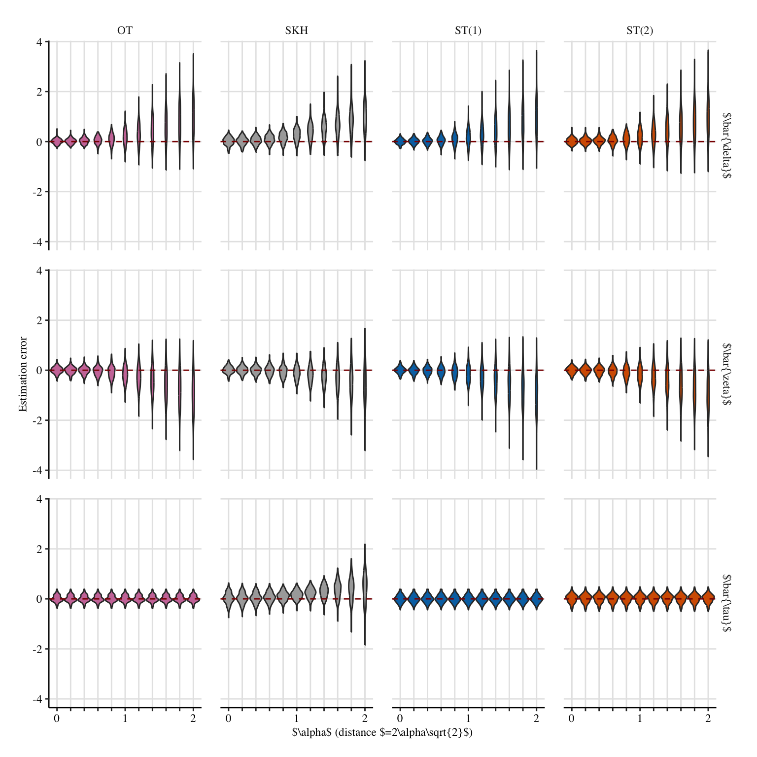
6.3 Varying the Proportion of 0s and 1s
In this section, we let the proportion of untreated/treated units vary from 5% of 0s to 95% of them. Note that we go back to the distance between the mean equal to 1, as in Chapter 5.
A visual representation of the samples that can be drawn from the DGP with different proportions 0s is shown in Figure 6.2
Codes to create the Figure.
set.seed(123)

alpha <- 1
mu0 <- -1
mu1 <- +1
r0 <- +.7
r1 <- -.5

# Generate data with alpha=0, alpha=1, alpha=2
data_alpha_10 <- gen_data(
  a = alpha, mu0 = mu0, mu1 = mu1, r0 = r0, r1 = r1,
  n0 = 50, n1 = 450
)
data_alpha_50 <- gen_data(
  a = alpha, mu0 = mu0, mu1 = mu1, r0 = r0, r1 = r1,
  n0 = 25, n1 = 475
)
data_alpha_90 <- gen_data(
  a = alpha, mu0 = mu0, mu1 = mu1, r0 = r0, r1 = r1,
  n0 = 450, n1 = 50
)


par(mar = c(2.1, 2.1, 2.1, 0.1), mfrow = c(1, 3))
x_lim <- c(-4, 4)
y_lim <- c(-4, 4)
cex_pts <- .4

# With 10%----
a <- 0

x_lab <- "Prop. 0s: $10\\%$"
if (export_tikz == FALSE) x_lab <- latex2exp::TeX(x_lab)

plot(
  data_alpha_10$X1[data_alpha_10$A == 0],
  data_alpha_10$X2[data_alpha_10$A == 0],
  pch = 16,
  cex = cex_pts,
  col = adjustcolor(colGpe0, alpha = .3),
  xlim = x_lim, ylim = y_lim,
  xlab = "", ylab = "",
  main = x_lab,
  family = font_family,
  axes = FALSE
)
axis(1, at = -3:3)
axis(2, at = -3:3)
title(xlab = "X1", ylab="X2", line=2, cex.lab=1.2, family = font_family)
points(
  data_alpha_10$X1[data_alpha_10$A == 1],
  data_alpha_10$X2[data_alpha_10$A == 1],
  col = adjustcolor(colGpe1, alpha = .3), pch = 16, cex = cex_pts
)

# True mean and covariance (scaled by 'a')
Mu0 <- rep(alpha * mu0, 2)
Mu1 <- rep(alpha * mu1, 2)
Sig0 <- matrix(c(1, r0, r0, 1), 2, 2)
Sig1 <- matrix(c(1, r1, r1, 1), 2, 2)


# Add ellipses
draw_ellipse(Mu0, Sig0, col = colGpe0, lty = 2)
draw_ellipse(Mu1, Sig1, col = colGpe1, lty = 2)

# With 50%----
a <- 1

x_lab <- "Prop. 0s: $50\\%$"
if (export_tikz == FALSE) x_lab <- latex2exp::TeX(x_lab)

plot(
  data_alpha_50$X1[data_alpha_50$A == 0],
  data_alpha_50$X2[data_alpha_50$A == 0],
  pch = 16, cex = cex_pts,
  col = adjustcolor(colGpe0, alpha = .3),
  xlim = x_lim, ylim = y_lim,
  xlab = "", ylab = "",
  main = x_lab,
  family = font_family,
  axes = FALSE
)
axis(1, at = -3:3)
axis(2, at = -3:3)
title(xlab = "X1", ylab="X2", line=2, cex.lab=1.2, family = font_family)
points(
  data_alpha_50$X1[data_alpha_50$A == 1],
  data_alpha_50$X2[data_alpha_50$A == 1],
  col = adjustcolor(colGpe1, alpha = .3), pch = 16, cex = cex_pts
)

# True mean and covariance (scaled by 'a')
Mu0 <- rep(alpha * mu0, 2)
Mu1 <- rep(alpha * mu1, 2)
Sig0 <- matrix(c(1, r0, r0, 1), 2, 2)
Sig1 <- matrix(c(1, r1, r1, 1), 2, 2)

# Add ellipses
draw_ellipse(Mu0, Sig0, col = colGpe0, lty = 2)
draw_ellipse(Mu1, Sig1, col = colGpe1, lty = 2)

# With 90%----
a <- 2

x_lab <- "Prop. 0s: $90\\%$"
if (export_tikz == FALSE) x_lab <- latex2exp::TeX(x_lab)

plot(
  data_alpha_90$X1[data_alpha_90$A == 0],
  data_alpha_90$X2[data_alpha_90$A == 0],
  pch = 16, cex = cex_pts,
  col = adjustcolor(colGpe0, alpha = .3),
  xlim = x_lim, ylim = y_lim,
  xlab = "", ylab = "",
  main = x_lab,
  family = font_family,
  axes = FALSE
)
axis(1, at = -3:3)
axis(2, at = -3:3)
title(xlab = "X1", ylab="X2", line=2, cex.lab=1.2, family = font_family)
points(
  data_alpha_90$X1[data_alpha_90$A == 1],
  data_alpha_90$X2[data_alpha_90$A == 1],
  col = adjustcolor(colGpe1, alpha = .3), pch = 16, cex = cex_pts
)

# True mean and covariance (scaled by 'a')
Mu0 <- rep(alpha * mu0, 2)
Mu1 <- rep(alpha * mu1, 2)
Sig0 <- matrix(c(1, r0, r0, 1), 2, 2)
Sig1 <- matrix(c(1, r1, r1, 1), 2, 2)

# Add ellipses
draw_ellipse(Mu0, Sig0, col = colGpe0, lty = 2)
draw_ellipse(Mu1, Sig1, col = colGpe1, lty = 2)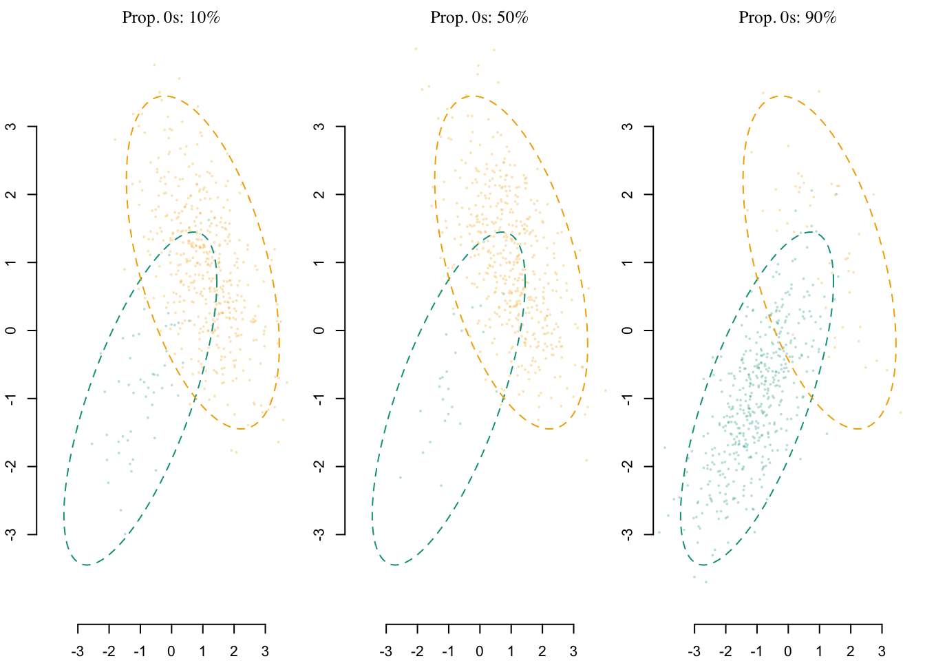
We define a grid with the different simulations.
grid_params <- expand_grid(
  prop_0 = seq(5, 95, by = 5)/100,
  mu0 = -1,
  mu1 = +1,
  r0 = +.7,
  r1 = -.5,
  a = 1,
  seed = seq_len(n_repl)
)
The simulations can be run in parallel, as follows.
The codes to run the simulations
# This chunk takes about XX minutes to run.
# We do not evaluate when compiling the document.
# Instead, we load previously obtained results.
library(pbapply)
library(parallel)
ncl <- detectCores()-1
(cl <- makeCluster(ncl))

clusterEvalQ(cl, {
  library(tidyverse)
  library(mnormt)
  library(expm)
  library(randomForest)
  library(fairadapt)
}) |>
  invisible()

clusterExport(
  cl = cl, c(
    "gen_data", "compute_ot_map", "apply_ot_transport",
    "transport_regul", "transport_many_to_one",
    "sequential_transport_12", "sequential_transport_21",
    "causal_effects_cf", "sim_f", "grid_params",
    "fairadapt_12", "fairadapt_21"
  )
)

res_sim_prop <- pbapply::pblapply(
  1:nrow(grid_params), function(i) {

    grid_params_current <- grid_params[i, ]

    n <- 500
    prop_0 <- grid_params_current$prop_0
    n0 <- prop_0 * n
    n1 <- n - n0
    mu0 <- grid_params_current$mu0
    mu1 <- grid_params_current$mu1
    r0 <- grid_params_current$r0
    r1 <- grid_params_current$r1
    a <- grid_params_current$a
    seed <- grid_params_current$seed

    sim_f(
      n0 = n0, n1 = n1,
      mu0 = mu0, mu1 = mu1,
      r0 = r0, r1 = r1,
      a = a, seed = seed
    ) |>
    mutate(prop_0 = prop_0)
}, cl = cl)


stopCluster(cl)
res_sim_prop <- list_rbind(res_sim_prop)

save(
    res_sim_prop,
    file = "../output/res_sim_prop-gaussian-mc.rda"
)
We load previously obtained results:
load("../output/res_sim_prop-gaussian-mc.rda")Codes to create the Figure.
a1 <- 2
a2 <- -1.5
export_pdf <- TRUE #FALSE

x_lab <- "Proportion of untreated"
y_lab <- "Distance to $\\bar\\tau$"

if (export_pdf == FALSE) {
  x_lab <- latex2exp::TeX(x_lab)
  y_lab <- latex2exp::TeX(y_lab)
}

data_plot <- res_sim_prop |>
  dplyr::select(
    n0, n1, seed, a, mu0, mu1, prop_0,
    tot_effect_med, tot_effect_ot, tot_effect_tmatch,
    tot_effect_skh, tot_effect_sot_12, tot_effect_sot_21,
    tot_effect_fairadapt_12_lin, tot_effect_fairadapt_21_lin
  ) |>
  pivot_longer(
    cols = c(
      tot_effect_med, tot_effect_ot, tot_effect_tmatch,
      tot_effect_skh, tot_effect_sot_12, tot_effect_sot_21,
      tot_effect_fairadapt_12_lin, tot_effect_fairadapt_21_lin
    ),
    names_to = "type", values_to = "tau"
  ) |>
  mutate(
    type = factor(
      type,
      levels = c(
        "tot_effect_med", "tot_effect_ot", "tot_effect_tmatch",
        "tot_effect_skh", "tot_effect_sot_12", "tot_effect_sot_21",
        "tot_effect_fairadapt_12_lin", "tot_effect_fairadapt_21_lin"
      ),
      labels = c("CM", "OT", "OT-M", "SKH", "ST(1)", "ST(2)", "FPT(1)", "FPT(2)")
    ),
    dist_to_causal_effect = (a1+a2) * (a*mu1 - a*mu0) + 3 - tau
  )

p <- ggplot(
  data = data_plot,
  mapping = aes(x = factor(prop_0), y = dist_to_causal_effect)
) +
  geom_violin(
    mapping = aes(fill = type)
  ) +
  geom_hline(yintercept = 0, colour = "darkred", linetype = "dashed") +
  theme_paper() +
  facet_wrap(~type, scales = "free_x", ncol = 2) +
  scale_fill_manual(
    NULL,
    values = c(
      "CM" = "#56B4E9",
      "OT" = colour_methods[["OT"]],
      "OT-M" = colour_methods[["OT-M"]],
      "SKH" = colour_methods[["skh"]],
      "ST(1)" =  colour_methods[["seq_1"]],
      "ST(2)" =  colour_methods[["seq_2"]],
      "FPT(1)" =  colour_methods[["fairadapt_1"]],
      "FPT(2)" =  colour_methods[["fairadapt_2"]]
    ),
    guide = "none",
  ) +
  theme(legend.position = "bottom") +
  labs(
    x = x_lab,
    y = y_lab,
  ) +
  scale_x_discrete(
    labels = ifelse(
      (unique(data_plot$prop_0)*100) %% 20 == 0,
      yes = unique(data_plot$prop_0), no = "")
  )

if (export_pdf == TRUE) {
  filename <- "gaussian-mc-prop-tau"
  ggplot2_to_pdf(
    plot = p + theme(panel.spacing = unit(0.4, "lines")),
    filename = filename, path = "figs/",
    width = 3.3, height = 3.5,
    crop = TRUE
  )

  system(paste0("pdfcrop figs/", filename, ".pdf figs/", filename, ".pdf"))
}

p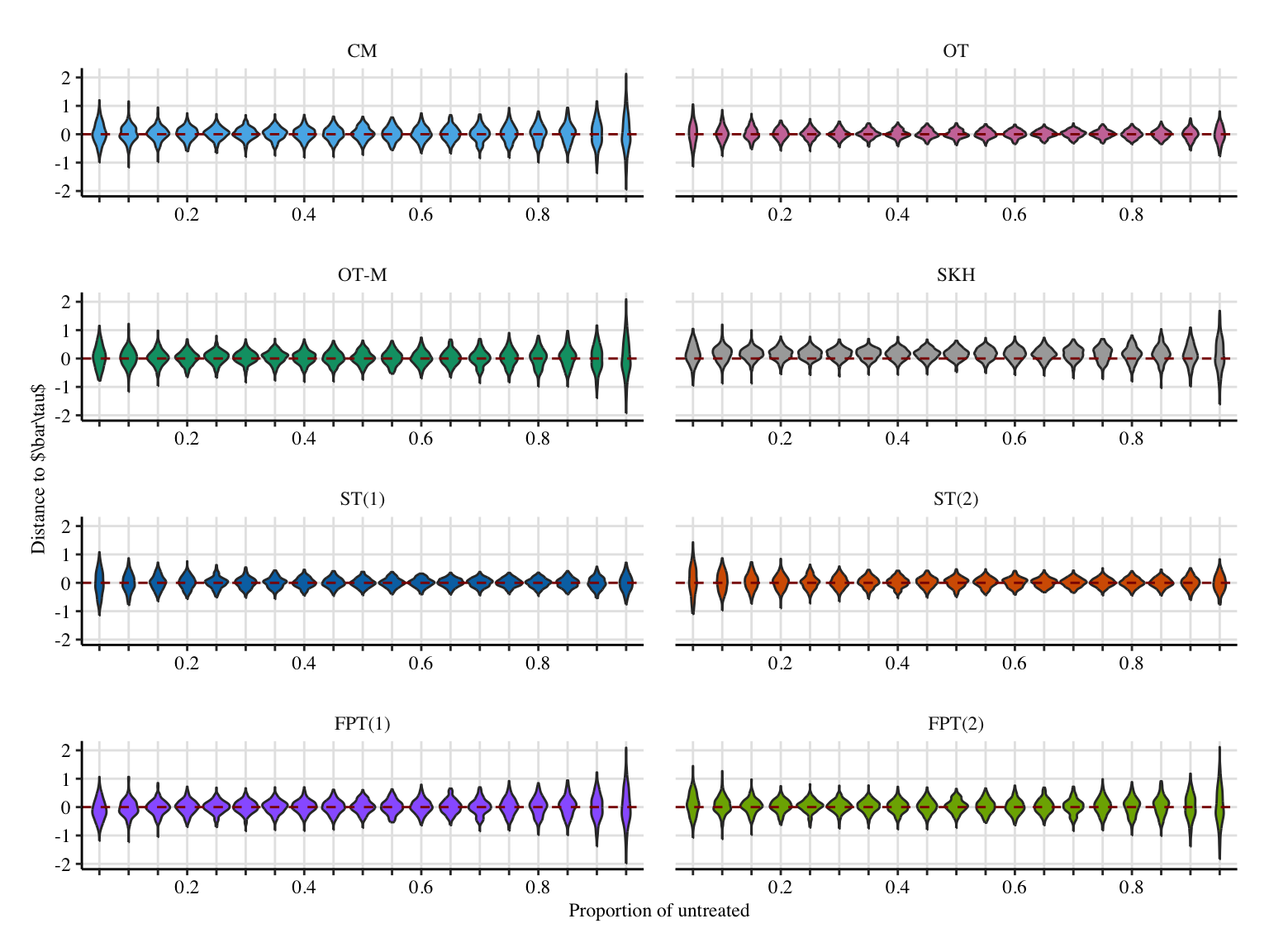
Codes to create the Figure.
a1 <- 2
a2 <- -1.5
export_pdf <- FALSE

x_lab <- "Proportion of untreated"
# y_lab <- "Distance to $\\bar\\delta(0)$"
y_lab <- "Distance to $\\bar\\delta$"

if (export_pdf == FALSE) {
  x_lab <- latex2exp::TeX(x_lab)
  y_lab <- latex2exp::TeX(y_lab)
}

data_plot <- res_sim_prop |>
  dplyr::select(
    n0, n1, seed, a, mu0, mu1, prop_0,
    delta_0_med, delta_0_ot, delta_0_tmatch,
    delta_0_skh, delta_0_sot_12, delta_0_sot_21,
    delta_0_fairadapt_12_lin, delta_0_fairadapt_21_lin
  ) |>
  pivot_longer(
    cols = c(
      delta_0_med, delta_0_ot, delta_0_tmatch,
      delta_0_skh, delta_0_sot_12, delta_0_sot_21,
      delta_0_fairadapt_12_lin, delta_0_fairadapt_21_lin
    ),
    names_to = "type", values_to = "val"
  ) |>
  mutate(
    type = factor(
      type,
      levels = c(
        "delta_0_med", "delta_0_ot", "delta_0_tmatch",
        "delta_0_skh", "delta_0_sot_12", "delta_0_sot_21",
        "delta_0_fairadapt_12_lin", "delta_0_fairadapt_21_lin"
      ),
      labels = c("CM", "OT", "OT-M", "SKH", "ST(1)", "ST(2)", "FPT(1)", "FPT(2)")
    ),
    dist_to_theo_val = ((a1+a2)*(mu1-mu0)) - val
  )

p <- ggplot(
  data = data_plot,
  mapping = aes(x = factor(prop_0), y = dist_to_theo_val)
) +
  geom_violin(
    mapping = aes(fill = type)
  ) +
  geom_hline(yintercept = 0, colour = "darkred", linetype = "dashed") +
  theme_paper() +
  facet_wrap(~type, scales = "free_x", ncol = 2) +
  scale_fill_manual(
    NULL,
    values = c(
      "CM" = "#56B4E9",
      "OT" = colour_methods[["OT"]],
      "OT-M" = colour_methods[["OT-M"]],
      "SKH" = colour_methods[["skh"]],
      "ST(1)" =  colour_methods[["seq_1"]],
      "ST(2)" =  colour_methods[["seq_2"]],
      "FPT(1)" =  colour_methods[["fairadapt_1"]],
      "FPT(2)" =  colour_methods[["fairadapt_2"]]
    ),
    guide = "none"
  ) +
  theme(legend.position = "bottom") +
  labs(
    x = x_lab,
    y = y_lab
  ) +
  scale_x_discrete(
    labels = ifelse(
      (unique(data_plot$prop_0)*100) %% 20 == 0,
      yes = unique(data_plot$prop_0), no = "")
  )

if (export_pdf == TRUE) {
  filename <- "gaussian-mc-prop-delta0"
  ggplot2_to_pdf(
    plot = p + theme(panel.spacing = unit(0.4, "lines")),
    filename = filename, path = "figs/",
    width = 3.3, height = 3.5,
    crop = TRUE
  )

  system(paste0("pdfcrop figs/", filename, ".pdf figs/", filename, ".pdf"))
}

p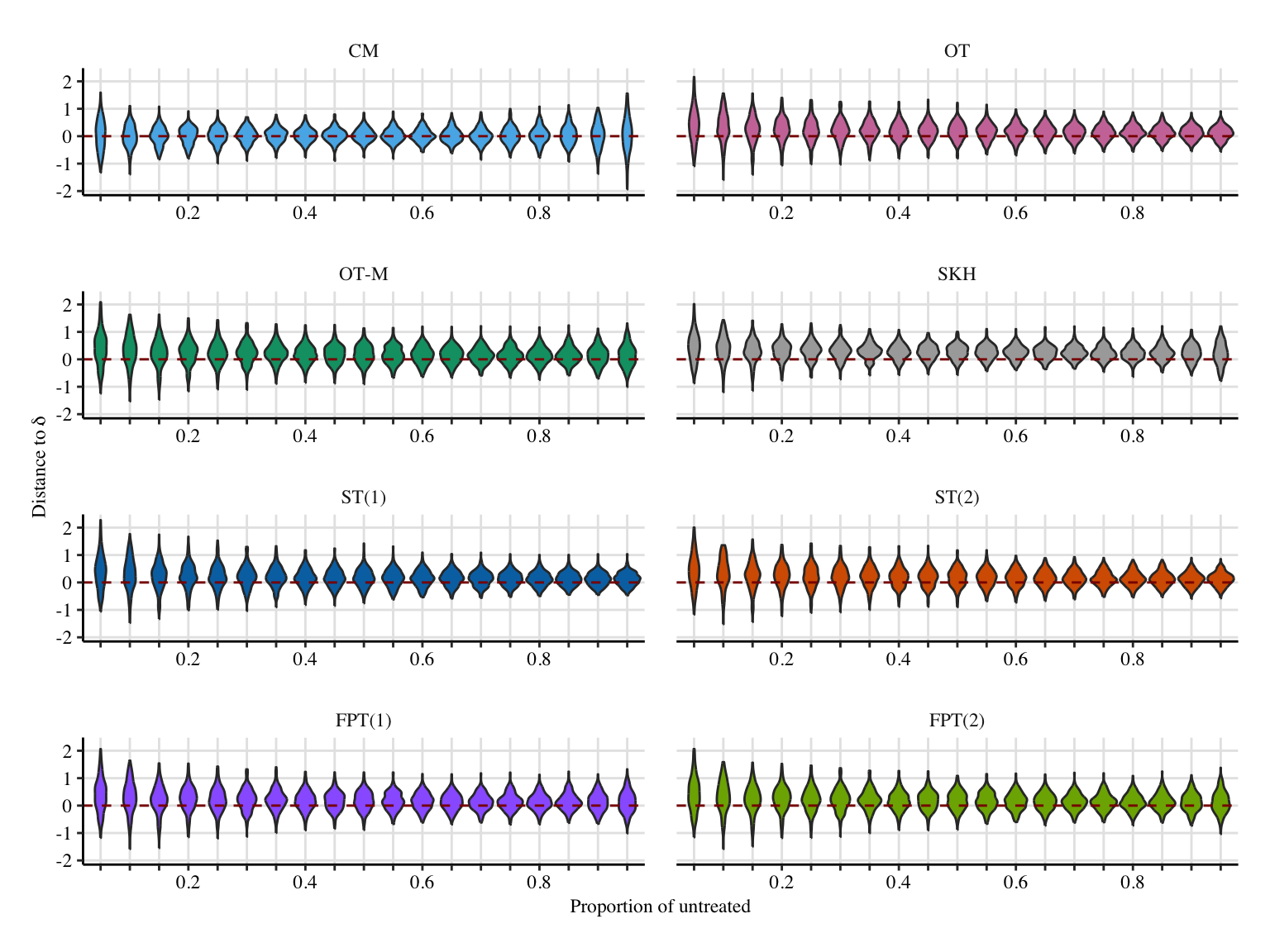
Codes to create the Figure.
data_plot <- res_sim_prop |>
  dplyr::select(
    n0, n1, seed, a, mu0, mu1, prop_0,
    delta_1_med, delta_1_ot, delta_1_tmatch,
    delta_1_skh, delta_1_sot_12, delta_1_sot_21,
    delta_1_fairadapt_12_lin, delta_1_fairadapt_21_lin
  ) |>
  pivot_longer(
    cols = c(
    delta_1_med, delta_1_ot, delta_1_tmatch,
    delta_1_skh, delta_1_sot_12, delta_1_sot_21,
    delta_1_fairadapt_12_lin, delta_1_fairadapt_21_lin),
    names_to = "type", values_to = "val"
  ) |>
  mutate(
    type = factor(
      type,
      levels = c(
        "delta_1_med", "delta_1_ot", "delta_1_tmatch",
        "delta_1_skh", "delta_1_sot_12", "delta_1_sot_21",
        "delta_1_fairadapt_12_lin", "delta_1_fairadapt_21_lin"
      ),
      labels = c("CM", "OT", "OT-M", "SKH", "ST(1)", "ST(2)", "FPT(1)", "FPT(2)")
    ),
    dist_to_theo_val = ((a1+a2)*(mu1-mu0)) - val
  )
ggplot(
  data = data_plot,
  mapping = aes(x = factor(prop_0), y = dist_to_theo_val)
) +
  geom_violin(
    mapping = aes(fill = type)
  ) +
  geom_hline(yintercept = 0, colour = "darkred", linetype = "dashed") +
  theme_paper() +
  facet_wrap(~type, scales = "free_x", ncol = 2) +
  scale_fill_manual(
    NULL,
    values = c(
      "CM" = "#56B4E9",
      "OT" = colour_methods[["OT"]],
      "OT-M" = colour_methods[["OT-M"]],
      "SKH" = colour_methods[["skh"]],
      "ST(1)" =  colour_methods[["seq_1"]],
      "ST(2)" =  colour_methods[["seq_2"]],
      "FPT(1)" =  colour_methods[["fairadapt_1"]],
      "FPT(2)" =  colour_methods[["fairadapt_2"]]
    ),
    guide = "none"
  ) +
  theme(legend.position = "bottom") +
  labs(
    x = "Proportion of 0",
    y = "Distance to theoretical natural indirect effect",
  ) +
  scale_x_discrete(
    labels = ifelse(
      (unique(data_plot$prop_0)*100) %% 10 == 0,
      yes = unique(data_plot$prop_0), no = "")
  )
Codes to create the Figure.
data_plot <- res_sim_prop |>
  dplyr::select(
    n0, n1, seed, a, mu0, mu1, prop_0,
    zeta_0_med, zeta_0_ot, zeta_0_tmatch,
    zeta_0_skh, zeta_0_sot_12, zeta_0_sot_21,
    zeta_0_fairadapt_12_lin, zeta_0_fairadapt_21_lin
  ) |>
  pivot_longer(
    cols = c(zeta_0_med, zeta_0_ot, zeta_0_tmatch,
    zeta_0_skh, zeta_0_sot_12, zeta_0_sot_21,
    zeta_0_fairadapt_12_lin, zeta_0_fairadapt_21_lin),
    names_to = "type", values_to = "val"
  ) |>
  mutate(
    type = factor(
      type,
      levels = c(
        "zeta_0_med", "zeta_0_ot", "zeta_0_tmatch",
        "zeta_0_skh", "zeta_0_sot_12", "zeta_0_sot_21",
        "zeta_0_fairadapt_12_lin", "zeta_0_fairadapt_21_lin"
      ),
      labels = c("CM", "OT", "OT-M", "SKH", "ST(1)", "ST(2)", "FPT(1)", "FPT(2)")
    ),
    dist_to_theo_val = 3 - val
  )
ggplot(
  data = data_plot,
  mapping = aes(x = factor(prop_0), y = dist_to_theo_val)
) +
  geom_violin(
    mapping = aes(fill = type)
  ) +
  geom_hline(yintercept = 0, colour = "darkred", linetype = "dashed") +
  theme_paper() +
  facet_wrap(~type, scales = "free_x", ncol = 2) +
  scale_fill_manual(
    NULL,
    values = c(
      "CM" = "#56B4E9",
      "OT" = colour_methods[["OT"]],
      "OT-M" = colour_methods[["OT-M"]],
      "SKH" = colour_methods[["skh"]],
      "ST(1)" =  colour_methods[["seq_1"]],
      "ST(2)" =  colour_methods[["seq_2"]],
      "FPT(1)" =  colour_methods[["fairadapt_1"]],
      "FPT(2)" =  colour_methods[["fairadapt_2"]]
    ),
    guide = "none"
  ) +
  theme(legend.position = "bottom") +
  labs(
    x = "Proportion of 0",
    y = "Distance to theoretical natural direct effect",
  ) +
  scale_x_discrete(
    labels = ifelse(
      (unique(data_plot$prop_0)*100) %% 10 == 0,
      yes = unique(data_plot$prop_0), no = "")
  )
Codes to create the Figure.
a1 <- 2
a2 <- -1.5
export_pdf <- FALSE

x_lab <- "Proportion of untreated"
# y_lab <- "Distance to $\\bar\\zeta(1)$"
y_lab <- "Distance to $\\bar\\zeta$"

if (export_pdf == FALSE) {
  x_lab <- latex2exp::TeX(x_lab)
  y_lab <- latex2exp::TeX(y_lab)
}

data_plot <- res_sim_prop |>
  dplyr::select(
    n0, n1, seed, a, mu0, mu1, prop_0,
    zeta_1_med, zeta_1_ot, zeta_1_tmatch,
    zeta_1_skh, zeta_1_sot_12, zeta_1_sot_21,
    zeta_1_fairadapt_12_lin, zeta_1_fairadapt_21_lin
  ) |>
  pivot_longer(
    cols = c(
      zeta_1_med, zeta_1_ot, zeta_1_tmatch,
      zeta_1_skh, zeta_1_sot_12, zeta_1_sot_21,
      zeta_1_fairadapt_12_lin, zeta_1_fairadapt_21_lin),
    names_to = "type", values_to = "val"
  ) |>
  mutate(
    type = factor(
      type,
      levels = c(
        "zeta_1_med", "zeta_1_ot", "zeta_1_tmatch",
        "zeta_1_skh", "zeta_1_sot_12", "zeta_1_sot_21",
        "zeta_1_fairadapt_12_lin", "zeta_1_fairadapt_21_lin"
      ),
      labels = c("CM", "OT", "OT-M", "SKH", "ST(1)", "ST(2)", "FPT(1)", "FPT(2)")
    ),
    dist_to_theo_val = 3 - val
  )
p <- ggplot(
  data = data_plot,
  mapping = aes(x = factor(prop_0), y = dist_to_theo_val)
) +
  geom_violin(
    mapping = aes(fill = type)
  ) +
  geom_hline(yintercept = 0, colour = "darkred", linetype = "dashed") +
  theme_paper() +
  facet_wrap(~type, scales = "free_x", ncol = 2) +
  scale_fill_manual(
    NULL,
    values = c(
      "CM" = "#56B4E9",
      "OT" = colour_methods[["OT"]],
      "OT-M" = colour_methods[["OT-M"]],
      "SKH" = colour_methods[["skh"]],
      "ST(1)" =  colour_methods[["seq_1"]],
      "ST(2)" =  colour_methods[["seq_2"]],
      "FPT(1)" =  colour_methods[["fairadapt_1"]],
      "FPT(2)" =  colour_methods[["fairadapt_2"]]
    ),
    guide = "none"
  ) +
  theme(legend.position = "bottom") +
  labs(
    x = x_lab,
    y = y_lab
  ) +
  scale_x_discrete(
    labels = ifelse(
      (unique(data_plot$prop_0)*100) %% 20 == 0,
      yes = unique(data_plot$prop_0), no = "")
  )

if (export_pdf == TRUE) {
  filename <- "gaussian-mc-prop-zeta1"
  ggplot2_to_pdf(
    plot = p + theme(panel.spacing = unit(0.4, "lines")),
    filename = filename, path = "figs/",
    width = 3.3, height = 3.5,
    crop = TRUE
  )

  system(paste0("pdfcrop figs/", filename, ".pdf figs/", filename, ".pdf"))
}

p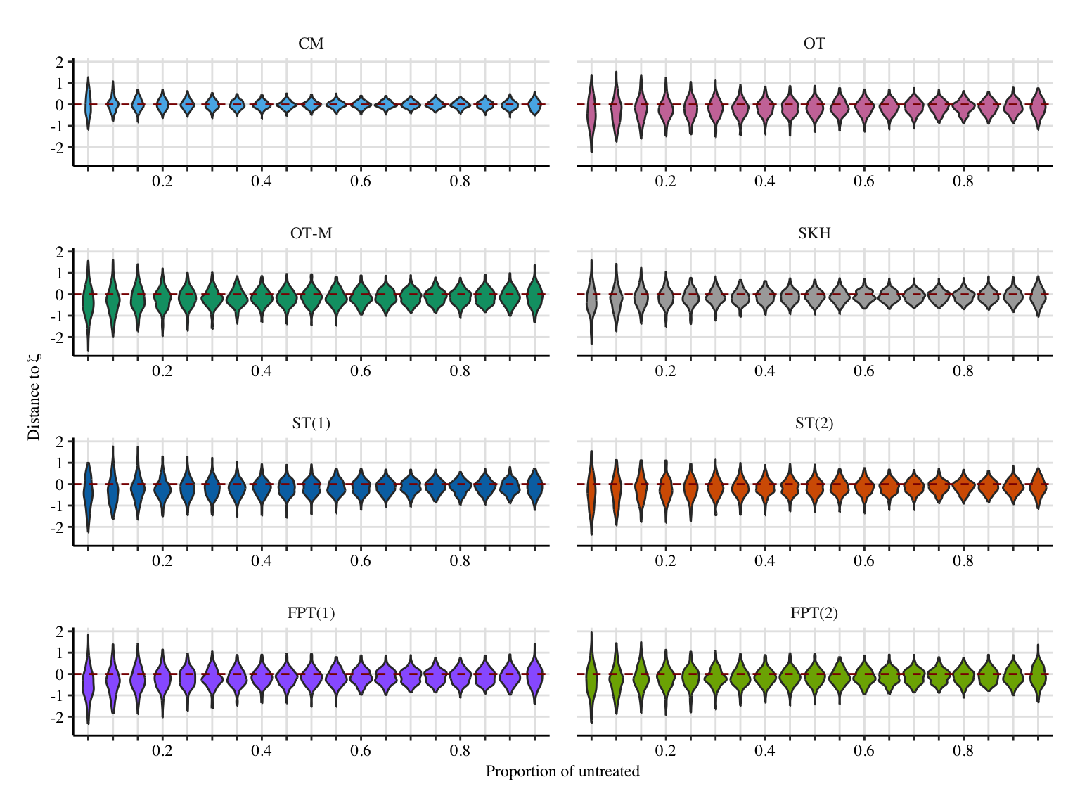
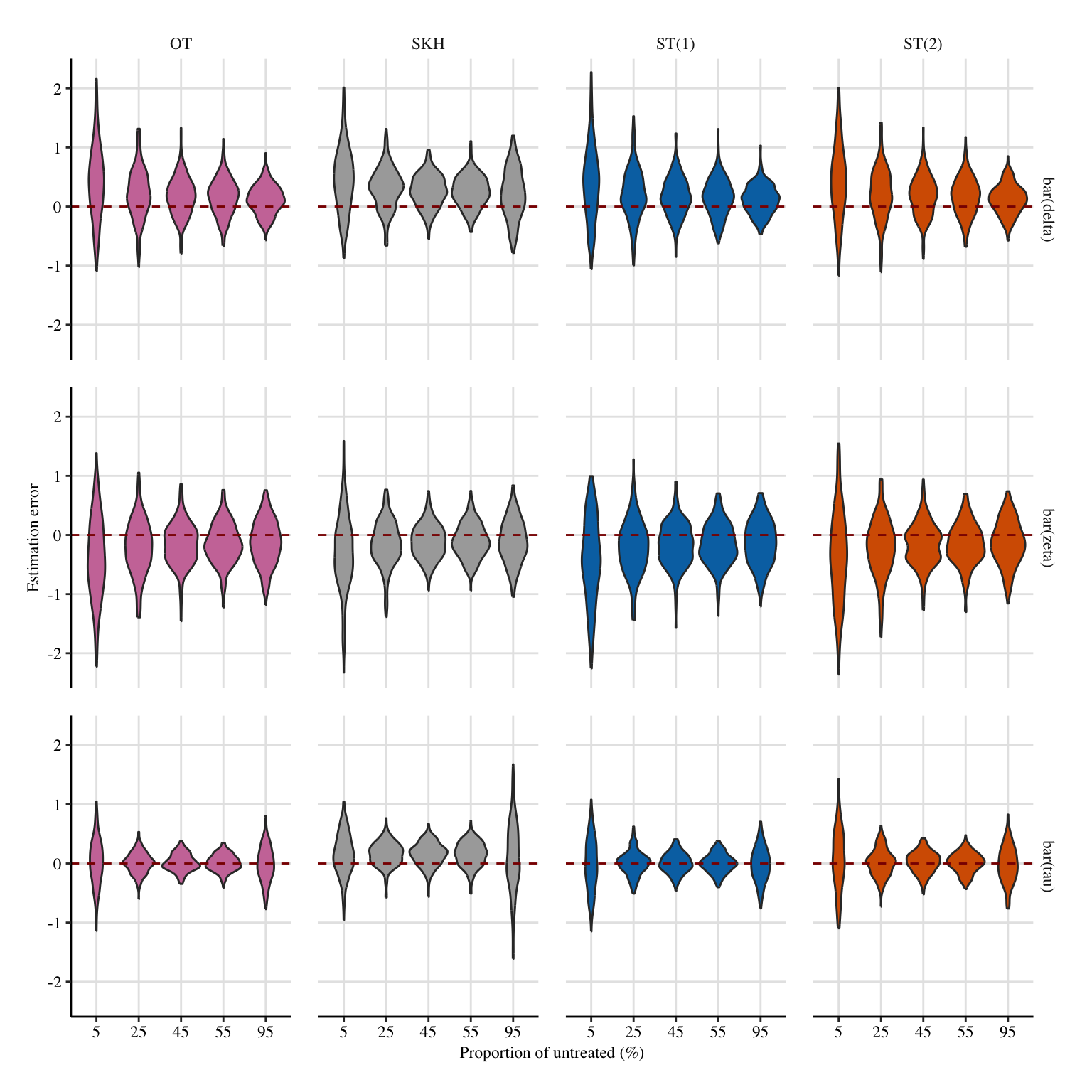
A more condensed figure, which focuses on \(\bar{\delta}(0)\), \(\bar{\zeta}(1)\), and \(\bar{\tau}\).
Codes to create the Figure.
a1 <- 2
a2 <- -1.5

x_lab <- "Proportion of untreated ($\\%$)"
y_lab <- "Estimation error"
# metrics_lab <- c("$\\bar{\\delta}(0)$", "$\\bar{\\zeta}(1)$", "$\\bar{\\tau}$")
metrics_lab <- c("$\\bar{\\delta}$", "$\\bar{\\zeta}$", "$\\bar{\\tau}$")


x_lab <- latex2exp::TeX(x_lab)
y_lab <- latex2exp::TeX(y_lab)
metrics_lab <- latex2exp::TeX(metrics_lab)


data_plot_tau <- res_sim_prop |>
  dplyr::select(
    n0, n1, seed, a, mu0, mu1, prop_0,
    tot_effect_med,
    tot_effect_fairadapt_12_lin, tot_effect_fairadapt_21_lin,
    tot_effect_ot, tot_effect_tmatch,
    tot_effect_skh, tot_effect_sot_12, tot_effect_sot_21
  ) |>
  pivot_longer(
    cols = c(
      tot_effect_med,
      tot_effect_fairadapt_12_lin, tot_effect_fairadapt_21_lin,
      tot_effect_ot, tot_effect_tmatch,
      tot_effect_skh, tot_effect_sot_12, tot_effect_sot_21
    ),
    names_to = "type", values_to = "tau"
  ) |>
  mutate(
    type = factor(
      type,
      levels = c(
        "tot_effect_med",
        "tot_effect_fairadapt_12_lin", "tot_effect_fairadapt_21_lin",
        "tot_effect_ot", "tot_effect_tmatch",
        "tot_effect_skh", "tot_effect_sot_12", "tot_effect_sot_21"
      ),
      labels = c("CM", "FPT(1)", "FPT(2)", "OT", "OT-M", "SKH", "ST(1)", "ST(2)")
    ),
    dist_to_causal_effect = (a1+a2) * (a*mu1 - a*mu0) + 3 - tau
  )

data_plot_delta0 <- res_sim_prop |>
  dplyr::select(
    n0, n1, seed, a, mu0, mu1, prop_0,
    delta_0_med,
    delta_0_fairadapt_12_lin, delta_0_fairadapt_21_lin,
    delta_0_ot, delta_0_tmatch,
    delta_0_skh, delta_0_sot_12, delta_0_sot_21
  ) |>
  pivot_longer(
    cols = c(
      delta_0_med,
      delta_0_fairadapt_12_lin, delta_0_fairadapt_21_lin,
      delta_0_ot, delta_0_tmatch,
      delta_0_skh, delta_0_sot_12, delta_0_sot_21
    ),
    names_to = "type", values_to = "val"
  ) |>
  mutate(
    type = factor(
      type,
      levels = c(
        "delta_0_med",
        "delta_0_fairadapt_12_lin", "delta_0_fairadapt_21_lin",
        "delta_0_ot", "delta_0_tmatch",
        "delta_0_skh", "delta_0_sot_12", "delta_0_sot_21"
      ),
      labels = c("CM", "FPT(1)", "FPT(2)", "OT", "OT-M", "SKH", "ST(1)", "ST(2)")
    ),
    dist_to_theo_val = ((a1+a2)*(mu1-mu0)) - val
  )

data_plot_zeta1 <- res_sim_prop |>
  dplyr::select(
    n0, n1, seed, a, mu0, mu1, prop_0,
    zeta_1_med,
    zeta_1_fairadapt_12_lin, zeta_1_fairadapt_21_lin,
    zeta_1_ot, zeta_1_tmatch,
    zeta_1_skh, zeta_1_sot_12, zeta_1_sot_21
  ) |>
  pivot_longer(
    cols = c(
      zeta_1_med,
      zeta_1_fairadapt_12_lin, zeta_1_fairadapt_21_lin,
      zeta_1_ot, zeta_1_tmatch,
      zeta_1_skh, zeta_1_sot_12, zeta_1_sot_21),
    names_to = "type", values_to = "val"
  ) |>
  mutate(
    type = factor(
      type,
      levels = c(
        "zeta_1_med",
        "zeta_1_fairadapt_12_lin", "zeta_1_fairadapt_21_lin",
        "zeta_1_ot", "zeta_1_tmatch",
        "zeta_1_skh", "zeta_1_sot_12", "zeta_1_sot_21"
      ),
      labels = c("CM", "FPT(1)", "FPT(2)", "OT", "OT-M", "SKH", "ST(1)", "ST(2)")
    ),
    dist_to_theo_val = 3 - val
  )

data_plot <- data_plot_tau |>
  rename(dist_tau = dist_to_causal_effect) |>
  left_join(
    data_plot_delta0 |>
      rename(
        delta0 = val,
        dist_delta0 = dist_to_theo_val
      ),
    by = c("n0", "n1", "seed", "a", "mu0", "mu1", "type", "prop_0")
  ) |>
  left_join(
    data_plot_zeta1 |>
      rename(
        zeta1 = val,
        dist_zeta1 = dist_to_theo_val
      ),
    by = c("n0", "n1", "seed", "a", "mu0", "mu1", "type", "prop_0")
  )

data_plot <- data_plot |> filter(prop_0 %in% seq(.05, .95, by =.1))


p <- ggplot(
  data = data_plot |> select(-tau, -delta0, -zeta1) |>
    pivot_longer(
      cols = c(dist_tau, dist_delta0, dist_zeta1),
      names_to = "metric",
      values_to = "dist"
    ) |>
    mutate(
      metric = factor(
        metric,
        levels = c("dist_delta0", "dist_zeta1", "dist_tau"),
        labels = metrics_lab
      )
    ),
  mapping = aes(x = factor(prop_0), y = dist)
) +
  geom_violin(
    mapping = aes(fill = type)
  ) +
  geom_hline(yintercept = 0, colour = "darkred", linetype = "dashed") +
  theme_paper() +
  facet_grid(metric ~ type, scales = "free_x") +
  scale_fill_manual(
    NULL,
    values = c(
      "CM" = "#56B4E9",
      "FPT(1)" =  colour_methods[["fairadapt_1"]],
      "FPT(2)" =  colour_methods[["fairadapt_2"]],
      "OT" = colour_methods[["OT"]],
      "OT-M" = colour_methods[["OT-M"]],
      "SKH" = colour_methods[["skh"]],
      "ST(1)" =  colour_methods[["seq_1"]],
      "ST(2)" =  colour_methods[["seq_2"]]
    ),
    guide = "none",
  ) +
  theme(legend.position = "bottom") +
  labs(
    x = x_lab,
    y = y_lab,
  ) +
  scale_x_discrete(
    labels = 100*unique(data_plot$prop_0)
  )

p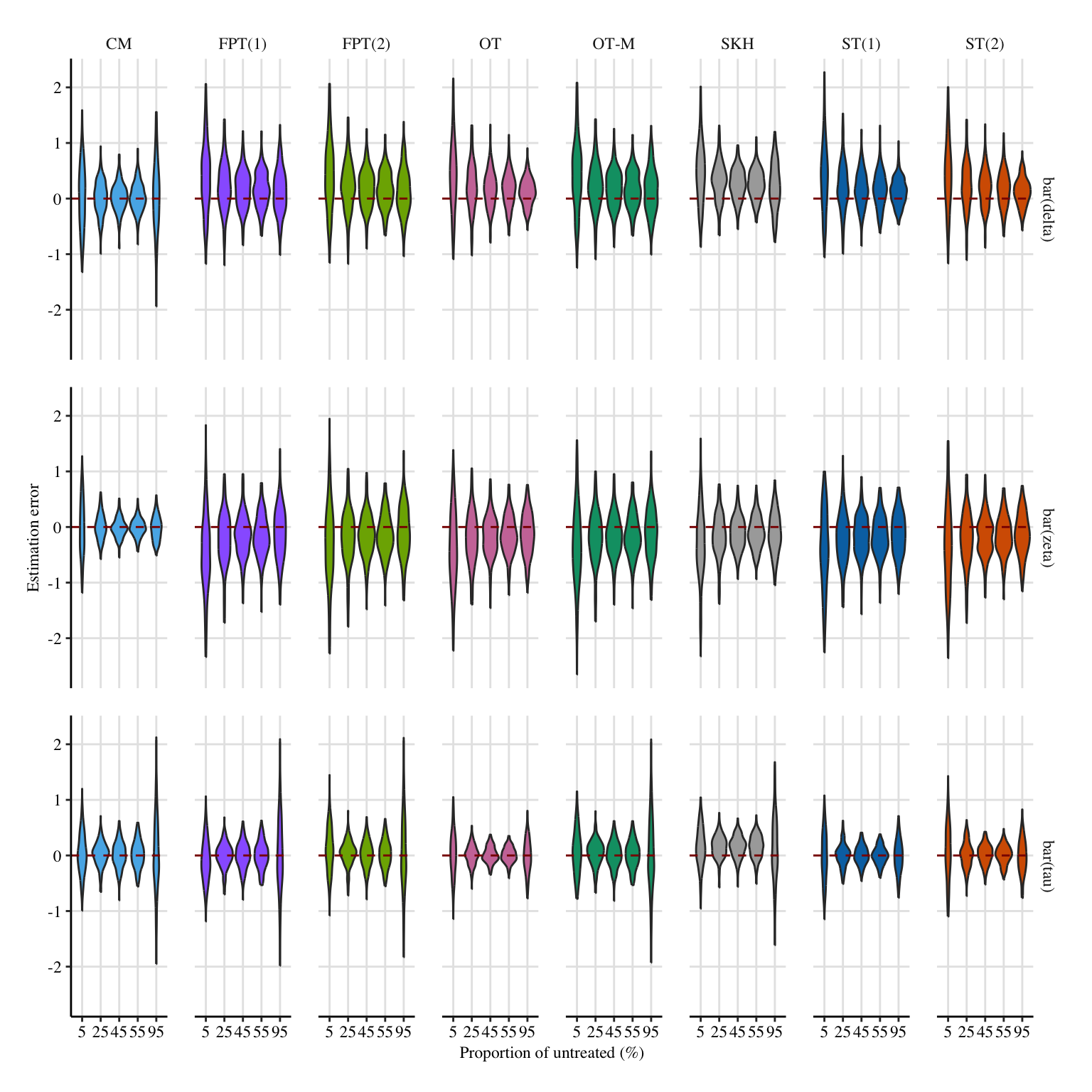
A shorter version of the graph for the paper.
Codes to create the Figure.
a1 <- 2
a2 <- -1.5
export_pdf <- FALSE

x_lab <- "Proportion of untreated ($\\%$)"
y_lab <- "Estimation error"
metrics_lab <- c("$\\bar{\\delta}$", "$\\bar{\\zeta}$", "$\\bar{\\tau}$")

if (export_pdf == FALSE) {
  x_lab <- latex2exp::TeX(x_lab)
  y_lab <- latex2exp::TeX(y_lab)
  metrics_lab <- latex2exp::TeX(metrics_lab)
}

data_plot <- data_plot_tau |>
  rename(dist_tau = dist_to_causal_effect) |>
  left_join(
    data_plot_delta0 |>
      rename(
        delta0 = val,
        dist_delta0 = dist_to_theo_val
      ),
    by = c("n0", "n1", "seed", "a", "mu0", "mu1", "type", "prop_0")
  ) |>
  left_join(
    data_plot_zeta1 |>
      rename(
        zeta1 = val,
        dist_zeta1 = dist_to_theo_val
      ),
    by = c("n0", "n1", "seed", "a", "mu0", "mu1", "type", "prop_0")
  )

data_plot <- data_plot |> filter(prop_0 %in% seq(.05, .95, by =.1)) |>
  filter(type %in% c("ST(1)", "ST(2)", "OT", "SKH", "OT"))


p <- ggplot(
  data = data_plot |> select(-tau, -delta0, -zeta1) |>
    pivot_longer(
      cols = c(dist_tau, dist_delta0, dist_zeta1),
      names_to = "metric",
      values_to = "dist"
    ) |>
    mutate(
      metric = factor(
        metric,
        levels = c("dist_delta0", "dist_zeta1", "dist_tau"),
        labels = metrics_lab
      )
    ),
  mapping = aes(x = factor(prop_0), y = dist)
) +
  geom_violin(
    mapping = aes(fill = type)
  ) +
  geom_hline(yintercept = 0, colour = "darkred", linetype = "dashed") +
  theme_paper() +
  facet_grid(metric ~ type, scales = "free_x") +
  scale_fill_manual(
    NULL,
    values = c(
      "CM" = "#56B4E9",
      "FPT(1)" =  colour_methods[["fairadapt_1"]],
      "FPT(2)" =  colour_methods[["fairadapt_2"]],
      "OT" = colour_methods[["OT"]],
      "OT-M" = colour_methods[["OT-M"]],
      "SKH" = colour_methods[["skh"]],
      "ST(1)" =  colour_methods[["seq_1"]],
      "ST(2)" =  colour_methods[["seq_2"]]
    ),
    guide = "none",
  ) +
  theme(legend.position = "bottom") +
  labs(
    x = x_lab,
    y = y_lab,
  ) +
  scale_x_discrete(
    labels = 100*unique(data_plot$prop_0)
  )

scale <- .77
if (export_pdf == TRUE) {
  filename <- "gaussian-mc-prop"
  ggplot2_to_pdf(
    plot = p + theme(panel.spacing = unit(0.4, "lines")) +
      theme(axis.text.x = element_text(size = rel(1))),
    filename = filename, path = "figs/",
    height = scale*3.6, width = scale*6,
    crop = TRUE
  )

  system(paste0("pdfcrop figs/", filename, ".pdf figs/", filename, ".pdf"))
}
p