8 Random Matching

Objectives

We show how random matching between individuals from two groups can be made to assign a counterfactual value for a categorical variable.

This method is not that used in our methodology, but it (hopefully) helps understanding how our approach differs.

Codes for graphical parameters

# col_categ <- c("#ffdd55","#944edf","#3fb3b2")
col_group <- c("#00A08A","#F2AD00", "#1b95e0")
col_categ <- c("#56B4E9", "#D55E00", "#CC79A7")
colA <- col_categ[1] ; colB <- col_categ[2] ; colC <- col_categ[3]
colGpe1 <- col_group[2]
colGpe0 <- col_group[1]
font_size <- 20
font_family <- "CMU Serif"

path <- "./figs/"

theme_ggtern_paper <- function(...) {
  font_family <- "CMU Serif"
  font_size <- 10
  theme(
    strip.background = element_rect(colour = "black", fill = NA),
    strip.text.x = element_text(colour = "black"),
    strip.text = ggtext::element_markdown(),
    text = element_text(family = font_family, size = unit(font_size, "pt")),
    axis.title = element_text(size = rel(1)),
    tern.axis.arrow.show = TRUE,
    tern.axis.arrow.sep = .13,
    tern.axis.vshift = .05,
    panel.border = element_rect(colour = NA)
  )
}

theme_ggtern <- function(...) {
  font_family <- "CMU Serif"
  font_size <- 20
  theme(
    strip.background = element_rect(colour = "black", fill = NA),
    strip.text.x = element_text(colour = "black"),
    strip.text = ggtext::element_markdown(),
    text = element_text(family = font_family, size = unit(font_size, "pt")),
    axis.title = element_text(size = rel(1)),
    tern.axis.arrow.show = TRUE,
    tern.axis.arrow.sep = .13,
    tern.axis.vshift = .05,
    panel.border = element_rect(colour = NA)
  )
}

theme_ggtern_minimal <- function(...) {
  font_family <- "CMU Serif"
  font_size <- 10
  theme(
    strip.background = element_rect(colour = "black", fill = NA),
    # strip.text.x = element_text(colour = "black"),
    # strip.text = ggtext::element_markdown(),
    text = element_text(family = font_family, size = unit(font_size, "pt")),
    axis.title = element_text(size = rel(1)),
    tern.axis.arrow.show = FALSE,
    tern.axis.arrow.sep = .13,
    tern.axis.vshift = .05,
    panel.border = element_rect(colour = NA),
    tern.axis.text.T = element_blank(),
    tern.axis.text.L = element_blank(),
    tern.axis.text.R = element_blank(),
    tern.axis.vshift = 0.2
  )
}


#' Theme for ggplot2
#'
#' @param ... Arguments passed to the theme function.
#' @export
#' @importFrom ggplot2 element_rect element_text element_blank element_line unit
#'   rel theme
#'
theme_paper <- function (...) {
  theme(
    text = element_text(family = font_family),
    plot.background = element_rect(fill = "transparent", color = NA),
    panel.background = element_rect(fill = "transparent", color = NA),
    # panel.border = element_rect(fill = NA, colour = "black", linewidth = 1),
    panel.border = element_blank(),
    # axis.line = element_line(color = "black"),
    axis.line <- element_blank(),
    axis.text = element_text(color = "black"),
    legend.text = element_text(size = rel(1)),
    legend.title = element_text(size = rel(1)),
    legend.background = element_rect(fill = "transparent", color = NULL),
    # legend.position = "bottom",
    # legend.direction = "horizontal",
    # legend.box = "vertical",
    legend.key = element_blank(),
    panel.spacing = unit(1, "lines"),
    panel.grid.major = element_line(colour = "grey90"),
    panel.grid.minor = element_blank(),
    plot.title = element_text(hjust = 0, size = rel(1), face = "bold"),
    plot.title.position = "plot",
    plot.margin = unit(c(1, 1, 1, 1), "lines"),
    strip.background = element_rect(fill = NA, colour = NA),
    strip.text = element_text(size = rel(1))
  )
}

\[ \definecolor{wongBlack}{RGB}{0,0,0} \definecolor{wongGold}{RGB}{230, 159, 0} \definecolor{wongLightBlue}{RGB}{86, 180, 233} \definecolor{wongGreen}{RGB}{0, 158, 115} \definecolor{wongYellow}{RGB}{240, 228, 66} \definecolor{wongBlue}{RGB}{0, 114, 178} \definecolor{wongOrange}{RGB}{213, 94, 0} \definecolor{wongPurple}{RGB}{204, 121, 167} %\definecolor{colA}{RGB}{255, 221, 85} %\definecolor{colB}{RGB}{148, 78, 223} %\definecolor{colC}{RGB}{63, 179, 178} \definecolor{colA}{RGB}{0, 114, 178} \definecolor{colB}{RGB}{213, 94, 0} \definecolor{colC}{RGB}{204, 121, 167} \definecolor{colGpeZero}{RGB}{0,160,138} \definecolor{colGpeUn}{RGB}{242, 173, 0} \]

library(dplyr)
library(tidyr)
library(stringr)
library(ggtern)
library(compositions)
library(ggalluvial)

Recall from Chapter 7 that \(a\in\{0,1\}\) denotes a binary treatment. Let \(x\in\mathcal{X}\) denote a mediator variable. The objective here is to obtain counterfactuals \((a=1,\boldsymbol{x}(1))\) for untreated units \((t=0,\boldsymbol{x})\), when the variable \(x\) is categorical.

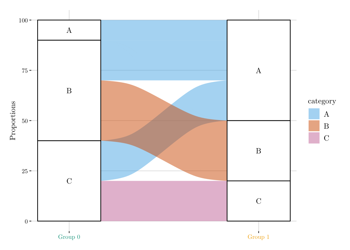
As in Chapter 7, consider the case where \(x\in\{A,B,C\}\) with the following group-wise proportions: \(\boldsymbol{p}_0 = (0.1, 0.5, 0.4)\) (untreated units) and \(\boldsymbol{p}_1 = (0.5, 0.3, 0.2)\) (treated units). The proportion in group 0 are shown in Figure 10.1.

8.1 Preliminary Example: 1-to-1 Random Matching

Let us generate a dummy data set with 100 individuals in both Group 0 and Group 1.

set.seed(1234)
n <- 100
n0 <- n1 <- n
p0 <- c(0.1, 0.5, 0.4)
p1 <- c(0.5, 0.3, 0.2)
# Sample category
x0 <- sample(c(rep("A", p0[1] * n0), rep("B", p0[2] * n0), rep("C", p0[3] * n0)), replace = FALSE)
x1 <- sample(c(rep("A", p1[1] * n1), rep("B", p1[2] * n1), rep("C", p1[3] * n1)), replace = FALSE)
cat_levels <- c("A", "B", "C")

A way to obtain the counterfactual for the categorical variable is to implement a 1-to-1 matching procedure.

Each category is assigned an arbitrary numeric value (e.g., \(A = 1\), \(B = 2\), \(C = 3\)), allowing us to define a cost matrix based on the absolute difference between encoded categories. That is, the cost of matching an individual from Group 0 with category \(x_{j0}\) to an individual from Group 1 with category \(x_{i1}\) is given by \(C_{ij} = |x_{i1} - x_{j0}|\).

A linear sum assignment problem can then be used to find the matching that minimizes the total cost across pairs.

The matched category from Group 1 is interpreted as the counterfactual category for the initial Group 0 individual.

We can compute the distance between the observations from Group 0 to Group 1, by setting numeric values to each category: A=1, B=2, C=3:

x0_index <- match(x0, cat_levels)
x1_index <- match(x1, cat_levels)
cost_matrix <- outer(x0_index, x1_index, function(i, j) abs(i - j))

The linear sum assignment problem is tackled with solve_LSAP() from {clue}.

library(clue)
assignment <- solve_LSAP(cost_matrix)

The mapping can be stored in a tibble.

tb_coupling <- tibble(
  x0 = x0,
  x1 = x1[assignment]
) |> 
  mutate(
    cost = abs(match(x0, cat_levels) - match(x1, cat_levels))
  )

We compute the number of observations from Group 0 matched with observations from Group 1 per category.

tb_coupling |> 
  group_by(x0, x1) |> 
  count() |> 
  group_by(x0) |> 
  mutate(prop_0 = 100 * n / sum(n)) |> 
  group_by(x1) |> 
  mutate(prop_1 = 100 * n / sum(n))

# A tibble: 5 × 5
# Groups:   x1 [3]
  x0    x1        n prop_0 prop_1
  <chr> <chr> <int>  <dbl>  <dbl>
1 A     A        10    100     20
2 B     A        20     40     40
3 B     B        30     60    100
4 C     A        20     50     40
5 C     C        20     50    100

Then, we can visualize the results, using an alluvial plot (Figure 8.1). All individuals in Group 0 with label A are matched directly to individuals in Group 1 with the same label. The remaining individuals in Group 1 labeled A are then matched to Group 0 individuals who originally had label B or C. This matching is performed probabilistically: among Group 0 individuals with label B, 60% retain their original label, and 40% are reclassified as A; among those with label C, 50% remain C, and 50% are reclassified as A.

Codes to create the Figure.

flow <- data.frame(
  depart = rep(LETTERS[1:3], 3),
  category = rep(LETTERS[1:3], each = 3),
  freq = as.vector(table(tb_coupling$x0, tb_coupling$x1))
)
p_1 <- ggplot(
  data = flow,
  mapping = aes(axis1 = depart, axis2 = category, y = freq)
) +
  geom_alluvium(aes(fill = category)) +
  geom_stratum() +
  scale_fill_manual(values = col_categ) +
  geom_text(
    stat = "stratum",
    mapping = aes(label = after_stat(stratum)),
    family = font_family
  ) +
  # scale_x_discrete(
  #   limits = c("Group 1", "Group 0"),
  #   expand = c(0.15, 0.05)
  # ) +
  scale_x_discrete(
    limits = c("Group 0", "Group 1"),
    labels = c(
      "Group 0" = str_c("<span style='color:", col_group[1], ";'>Group 0</span>"),
      "Group 1" = str_c("<span style='color:", col_group[2], ";'>Group 1</span>")
    ),
    expand = c(0.15, 0.05)
  ) +
  ylab("Proportions") + 
  scale_y_continuous(transform = ) +
  # theme_minimal(base_size = font_size, base_family = font_family) +
  theme_paper() +
  theme(
    axis.text.x = ggtext::element_markdown()
  )
p_1

Figure 8.1: Matching individuals given a categorical variable.

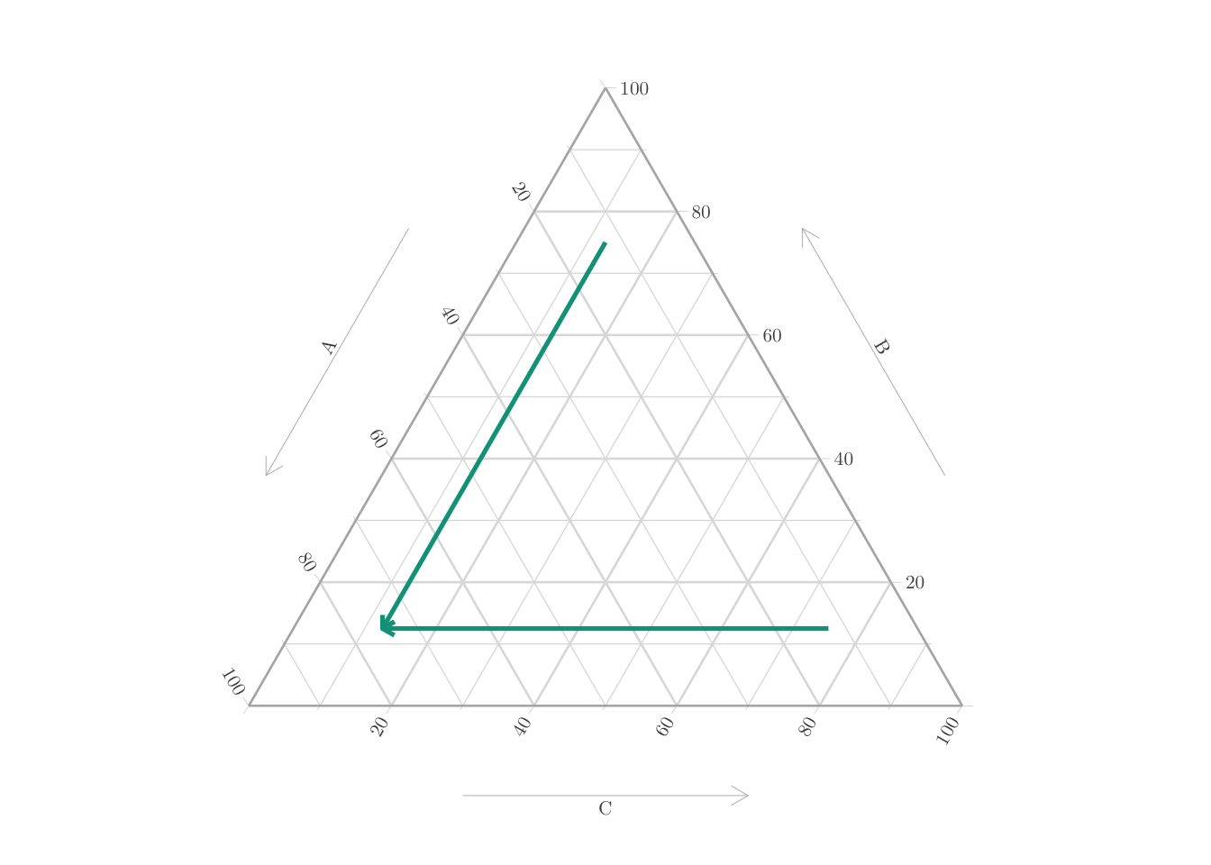
This can also be visualized on a ternary plot (Figure 8.2).

Codes to create the Figure.

# Create interpolated values using McCann (1997) displacement
f_line_simplex <- function(x, 
                           y, 
                           lgt = 601) {
  
  zx <- as.numeric(clr(x))[1:2]
  zy <- as.numeric(clr(y))[1:2]
  t <- seq(0, 1, length = lgt)
  
  tx <- cbind(
    (1 - t) * zx[1] + t * zy[1], 
    (1 - t) * zx[2] + t * zy[2]
  )
  tx <- cbind(tx, -(tx[, 1] + tx[, 2]))
  df <- as.data.frame(matrix(as.numeric(clrInv(tx)), lgt, 3))
  names(df) <- c("A","B","C")
  
  df
}

# dummy dataset to create an empty ternary plot
SB <- tibble(
  A = c(0.2, 0.3, 0.5, 0.6),
  B = c(0.3, 0.4, 0.2, 0.1),
  C = 1 - c(0.2, 0.3, 0.5, 0.6) - c(0.3, 0.4, 0.2, 0.1),
  group = c("0", "0", "1", "1")
)

p_2 <- ggtern(data = SB, aes(x = A, y = B, z = C)) +
  scale_colour_manual(name = "group", values = col_group) +
  guides(
    colour = guide_legend(
      override.aes = list(
        linetype = "solid",
        shape = NA,
        size = 1.5,
        alpha = 1
      )
    )
  ) +
  theme_light(base_size = font_size, base_family = font_family) +
  theme_ggtern_paper() +
  theme(
    legend.title = element_text(size = font_size),
    legend.text = element_text(size = font_size)
    # tern.axis.hshift = .10
  ) +
  theme_latex(TRUE) +
  theme_hidetitles()


p_2 <- p_2 + 
  geom_text(mapping = aes(x = 0.9, y = 0.06, z = 0.08), label = p1[1], color = col_group[2], family = font_family, size = font_size-3, size.unit = "pt") +
  geom_text(mapping = aes(x = 0.09, y = 0.9, z = 0.09), label = p1[2], color = col_group[2], family = font_family, size = font_size-3, size.unit = "pt") +
  geom_text(mapping = aes(x = 0.08, y = 0.06, z = 0.9), label = p1[3], color = col_group[2], family = font_family, size = font_size-3, size.unit = "pt") + 
  geom_text(mapping = aes(x = 0.3, y = 0.1, z = 0.11), label = p0[1], color = col_group[1], family = font_family, size = font_size-3, size.unit = "pt") +
  geom_text(mapping = aes(x = 0.15, y = 0.65, z = 0.25), label = p0[2], color = col_group[1], family = font_family, size = font_size-3, size.unit = "pt") +
  geom_text(mapping = aes(x = 0.1, y = 0.2, z = 0.8), label = p0[3], color = col_group[1], family = font_family, size = font_size-3, size.unit = "pt") 


Li1 <- f_line_simplex(x = c(.75, .125, .125), y = c(.125, .125, .75), lgt = 2)
Li2 <- f_line_simplex(x = c(.75, .125, .125), y = c(.125, .75, .125), lgt = 2)
p_2 <- p_2 + 
  geom_line(
    data = Li2, aes(x = A, y = B, z = C), 
    color = col_group[1], linwidth = .6,
    arrow = arrow(length=unit(0.20,"cm"))
  ) + 
  geom_line(
    data = Li1, aes(x = A, y = B, z = C), 
    color = col_group[1], linwidth = .6,
    arrow = arrow(length=unit(0.20,"cm"))
  ) 
p_2

Figure 8.2: Matching individuals given a categorical variable, on a Ternary plot.

Codes to export the figures in PDF.

p_matching_indiv <- cowplot::plot_grid(
  ggplotGrob(
    p_1 +
      # Remove top/bottom margin
      theme(
        plot.margin = ggplot2::margin(t = 0, r = 0, b = 0, l = 0)
      )
  ),
  # table_grob,
  ggplotGrob(
    p_2 +
      # Remove top/bottom margin
      theme(
        plot.background = element_rect(fill = "transparent", color = NA),
        plot.margin = ggplot2::margin(t = 0, r = 0, b = 0, l = 0)
      )
  ),
  rel_widths = c(1.4,1),
  ncol = 2
)

p_matching_indiv

filename <- "ternary-categ-matching-indiv"
ggsave(
  p_matching_indiv, file = str_c(path, filename, ".pdf"),
  height = 2*1.75, width = 3.75*1.75,
  family = font_family,
  device = cairo_pdf
)
# Crop PDF
system(paste0("pdfcrop ", path, filename, ".pdf ", path, filename, ".pdf"))

Rather than randomly matching individuals, we can use optimal transport to do the assignment. In Chapter 9, we begin by arbitrarily assigning numerical values to each category and computing pairwise distances based on these values. In contrast, Chapter 10 relies on an which consists in representing the categorical variable in the probability simplex, using probability vectors that reflect the likelihood of each category.