library(tidyverse)
# remotes::install_github(
#   repo = "fer-agathe/sequential_transport", subdir = "seqtransfairness"
# )
library(seqtransfairness)
# remotes::install_github(repo = "fer-agathe/transport-simplex")
library(transportsimplex)
library(randomForest)
library(fairadapt)
library(grf)
library(cluster)

# Also required:
# install.packages(mlr3fairness)14 Compas
Objectives
In this page, we calculate the average total causal effect, the average natural direct effect and the causal mediation effect (or indirect effect) of COMPAS dataset assuming a known causal graph. We compare three methodologies to estimate those effects:
- Using Optimal Transport (OT) to first derive counterfactuals at the individual level and then, averaging over all the individuals in the dataset,
- Using Sequential Transport (ST) to first derive counterfactuals at the individual level and then, averaging over all the individuals in the dataset,
- Using LSEM from causal mediation analysis that fits linear models to estimate the different average causal effects.
\[ \definecolor{wongBlack}{RGB}{0,0,0} \definecolor{wongGold}{RGB}{230, 159, 0} \definecolor{wongLightBlue}{RGB}{86, 180, 233} \definecolor{wongGreen}{RGB}{0, 158, 115} \definecolor{wongYellow}{RGB}{240, 228, 66} \definecolor{wongBlue}{RGB}{0, 114, 178} \definecolor{wongOrange}{RGB}{213, 94, 0} \definecolor{wongPurple}{RGB}{204, 121, 167} \definecolor{colA}{RGB}{255, 221, 85} \definecolor{colB}{RGB}{148, 78, 223} \definecolor{colC}{RGB}{63, 179, 178} \definecolor{colGpeZero}{RGB}{127, 23, 14} \definecolor{colGpeUn}{RGB}{27, 149, 224} \]
Codes for graphical parameters.
library(extrafont, quietly = TRUE)
font_family <- "CMU Serif"


path <- "./figs/"
if (!dir.exists(path)) dir.create(path)
We load the functions that will allow us to build the counterfactuals (see Chapter 4):
source("../scripts/functions.R")14.1 Data
We load the COMPAS dataset that is available in the {fairadapt} package.
data(compas, package = "fairadapt")The outcome variable is binary here: whether the defendant is rearrested at any time. The “treatment” \(A\) will be the sensitive attribute, race. In the data compiled in {fairadapt}, race is defined as White (which we will consider as \(A=1\)) and Non-White (which we will consider as \(A=0\)). The idea is to build counterfactuals for non-white people to ask questions such as “had this non-white individual been white, what would the prediction of an algorithm modeling recidivism be?”.
To train the predictive model of recidivism, we will use the following covariates: the age, the prior criminal records of defendants, and the charge degree (felony or misdemeanor).
tb <- compas |>
  as_tibble() |>
  select(
    race, # sensitive
    age,
    priors_count, # The prior criminal records of defendants.
    c_charge_degree, # F: Felony M: Misdemeanor
    is_recid = two_year_recid # outcome
  ) |>
  mutate(
   race = ifelse(race == "Non-White", 0, 1), # non-white indiv. as "untreated"
)dim(tb)[1] 7214 5summary(tb) race age priors_count c_charge_degree
Min. :0.0000 Min. :18.00 Min. : 0.000 F:4666
1st Qu.:0.0000 1st Qu.:25.00 1st Qu.: 0.000 M:2548
Median :0.0000 Median :31.00 Median : 2.000
Mean :0.3402 Mean :34.82 Mean : 3.472
3rd Qu.:1.0000 3rd Qu.:42.00 3rd Qu.: 5.000
Max. :1.0000 Max. :96.00 Max. :38.000
is_recid
Min. :0.0000
1st Qu.:0.0000
Median :0.0000
Mean :0.4507
3rd Qu.:1.0000
Max. :1.0000 #write.csv(tb, "compas.csv", row.names = FALSE)We assume the DAG shown in Figure 14.1.
variables <- c("race",
               "age", "priors_count", "c_charge_degree",
               "is_recid")
# Row: outgoing arrow
adj <- matrix(
  # S  1  2  3  Y
  c(0, 1, 1, 1, 1,# S
    0, 0, 1, 1, 1,# 1 (age)
    0, 0, 0, 0, 1,# 2 (priors_count)
    0, 0, 0, 0, 1,# 3 (c_charge_degree)
    0, 0, 0, 0, 0 # Y
  ),
  ncol = length(variables),
  dimnames = rep(list(variables), 2),
  byrow = TRUE
)

causal_graph <- fairadapt::graphModel(adj)
plot(causal_graph)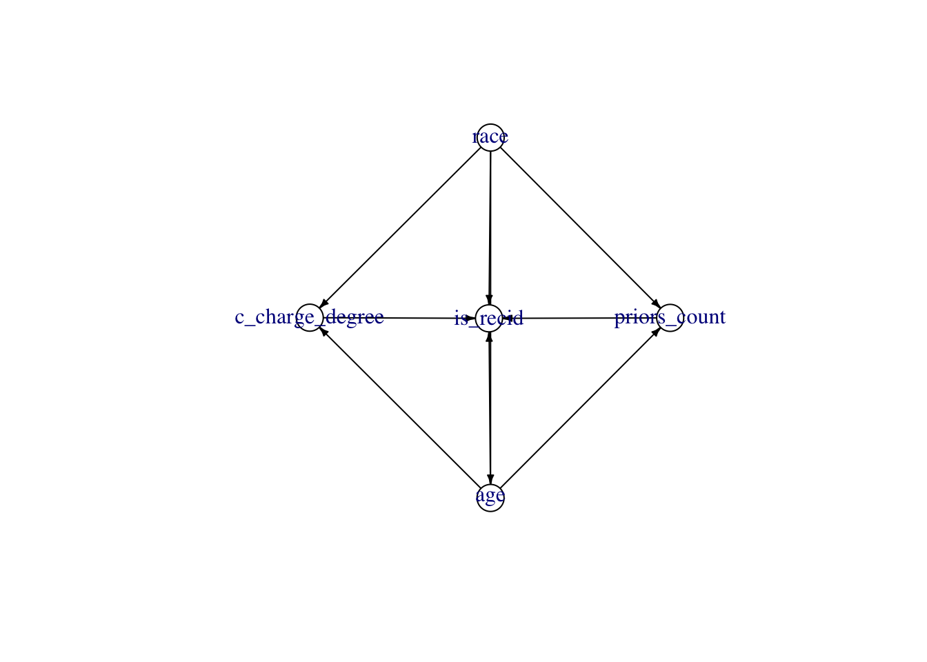
14.2 Counterfactuals
Let us set a seed for reproducibility.
seed <- 1234
set.seed(seed)
A_name <- "race" # treatment name
Y_name <- "is_recid" # outcome name
A_untreated <- 0
A <- tb[[A_name]]
ind_untreated <- which(A == A_untreated)
tb_untreated <- tb[ind_untreated, ]
tb_treated <- tb[-ind_untreated, ]Let us follow the DAG from Figure 14.1 and build the counterfactuals of non-white individuals: we thus transport individuals from \(A=0\) to \(A=1\), using the predictions on the test set.
14.2.1 Multivariate Optimal Transport
We apply multivariate optimal transport (OT), following the methodology developed in De Lara et al. (2024).
tb_untreated_wo_A <- tb_untreated[ , !(names(tb_untreated) %in% A_name)]
tb_treated_wo_A <- tb_treated[ , !(names(tb_treated) %in% A_name)]
n0 <- nrow(tb_untreated_wo_A)
n1 <- nrow(tb_treated_wo_A)
y0 <- tb_untreated_wo_A[[Y_name]]
y1 <- tb_treated_wo_A[[Y_name]]
X0 <- tb_untreated_wo_A[ , !(names(tb_untreated_wo_A) %in% Y_name)]
X1 <- tb_treated_wo_A[ , !(names(tb_treated_wo_A) %in% Y_name)]
To apply Optimal Transport on the COMPAS dataset, we first need to one-hot the categorical variables.
num_cols <- names(X0)[sapply(X0, is.numeric)]
cat_cols <- names(X0)[sapply(X0, function(col) is.factor(col) || is.character(col))]
X0_num <- X0[ , num_cols]
X1_num <- X1[ , num_cols]
X0_cat <- X0[ , cat_cols]
X1_cat <- X1[ , cat_cols]

cat_counts <- sapply(X0[ , cat_cols], function(col) length(unique(col)))
Categorical variables are one-hot encoded:
library(caret)
X0_cat_encoded <- list()
X1_cat_encoded <- list()
for (col in cat_cols) {
  # One-hot encoding with dummyVars
  formula <- as.formula(paste("~", col))
  dummies <- dummyVars(formula, data = X0_cat)

  # Dummy variable
  dummy_0 <- predict(dummies, newdata = X0_cat) %>% as.data.frame()
  dummy_1 <- predict(dummies, newdata = X1_cat) %>% as.data.frame()

  # Scaling
  dummy_0_scaled <- scale(dummy_0)
  dummy_1_scaled <- scale(dummy_1)

  dummy_0_df <- as.data.frame(dummy_0_scaled)
  dummy_1_df <- as.data.frame(dummy_1_scaled)

  # Aling categories in both treated/untreated groups
  all_cols <- union(colnames(dummy_0_df), colnames(dummy_1_df))
  dummy_0_df <- dummy_0_df %>% mutate(across(.fns = identity)) %>% select(all_of(all_cols)) %>% replace(is.na(.), 0)
  dummy_1_df <- dummy_1_df %>% mutate(across(.fns = identity)) %>% select(all_of(all_cols)) %>% replace(is.na(.), 0)

  # Sauvegarde dans les listes
  X0_cat_encoded[[col]] <- dummy_0_df
  X1_cat_encoded[[col]] <- dummy_1_df
}
We calculate Euclidean distance for numerical variables.
# library(proxy)
num_dist <- proxy::dist(x = X0_num, y = X1_num, method = "Euclidean")
num_dist <- as.matrix(num_dist)
For categorical variables, we use the Hamming distance.
cat_dists <- list()
for (col in cat_cols) {
  mat_0 <- as.matrix(X0_cat_encoded[[col]])
  mat_1 <- as.matrix(X1_cat_encoded[[col]])
  dist_mat <- proxy::dist(x = mat_0, y = mat_1, method = "Euclidean")
  cat_dists[[col]] <- as.matrix(dist_mat)
}
Then we need to combine the two distance matrices. We use weights equal to the proportion of numerical variables and the proportion of categorical variables, respectively for distances based on numerical and categorical variables.
combined_cost <- num_dist
for (i in seq_along(cat_dists)) {
  combined_cost <- combined_cost + cat_dists[[i]]
}
Then, we can compute the transport map:
# Uniform weights (equal mass)
w0 <- rep(1 / n0, n0)
w1 <- rep(1 / n1, n1)
# Compute transport plan
transport_res <- transport::transport(
  a = w0,
  b = w1,
  costm = combined_cost,
  method = "shortsimplex"
)

transport_plan <- matrix(0, nrow = n0, ncol = n1)
for(i in seq_len(nrow(transport_res))) {
  transport_plan[transport_res$from[i], transport_res$to[i]] <- transport_res$mass[i]
}
We first transport the numerical variables.
num_transported <- n0 * (transport_plan %*% as.matrix(X1_num))Then, we transport the categorical variables with label reconstruction (not perfect here).
cat_transported <- list()
for (col in cat_cols) {
  cat_probs <- transport_plan %*% as.matrix(X1_cat_encoded[[col]])
  cat_encoded_columns <- colnames(X1_cat_encoded[[col]])
  # For each obs., we take the index with the maximum value (approx. proba)
  max_indices <- apply(cat_probs, 1, which.max)
  prefix_pattern <- paste0("^", col, "\\.")
  cat_transported[[col]] <- sapply(max_indices, function(x) sub(prefix_pattern, "", cat_encoded_columns[x]))
}
We can now store the results into a tibble.
tb_ot_transported <- as_tibble(num_transported)
for (col in cat_cols) {
  tb_ot_transported[[col]] <- cat_transported[[col]]
}

save(tb_ot_transported, file = "../output/ot-compas.rda")
# Load tb_ot_transported
load("../output/ot-compas.rda")
tb_ot_transported <- tb_ot_transported |>
mutate(c_charge_degree = as.factor(c_charge_degree))
tb_ot_transported <- as.list(tb_ot_transported)14.2.2 Penalized Optimal Transport
We can directly compute the transport map using Sinkhorn penalty.
# Compute transport plan
sinkhorn_transport_res <- T4transport::sinkhornD(
  combined_cost, wx = w0, wy = w1, lambda = 0.1
)

sinkhorn_transport_plan <- sinkhorn_transport_res$plan
We first transport the numerical variables.
num_sinkhorn_transported <- n0 * (sinkhorn_transport_plan %*% as.matrix(X1_num))Then, we transport the categorical variables with label reconstruction (not perfect here).
cat_sinkhorn_transported <- list()
for (col in cat_cols) {
  cat_probs <- sinkhorn_transport_plan %*% as.matrix(X1_cat_encoded[[col]])
  cat_encoded_columns <- colnames(X1_cat_encoded[[col]])
  # For each obs., we take the index with the maximum value (approx. proba)
  max_indices <- apply(cat_probs, 1, which.max)
  prefix_pattern <- paste0("^", col, "\\.")
  cat_sinkhorn_transported[[col]] <- sapply(max_indices, function(x) sub(prefix_pattern, "", cat_encoded_columns[x]))
}
We can now store the results into a tibble.
tb_sinkhorn_transported <- as_tibble(num_sinkhorn_transported)
for (col in cat_cols) {
  tb_sinkhorn_transported[[col]] <- cat_sinkhorn_transported[[col]]
}

save(tb_sinkhorn_transported, file = "../output/sinkhorn-compas.rda")
# Load tb_sinkhorn_transported
load("../output/sinkhorn-compas.rda")
tb_sinkhorn_transported <- tb_sinkhorn_transported |>
mutate(c_charge_degree = as.factor(c_charge_degree))
tb_sinkhorn_transported <- as.list(tb_sinkhorn_transported)14.2.3 Sequential Transport
We call the seq_trans() function (see Chapter 4) function to build the counterfactuals of Black individuals. The estimations are done using parallel computation.
library(pbapply)
library(parallel)
ncl <- detectCores()-1
(cl <- makeCluster(ncl))
socket cluster with 9 nodes on host 'localhost'clusterEvalQ(cl, {
library(transportsimplex)
}) |>
invisible()
A_name <- "race" # treatment name
Y_name <- "is_recid" # outcome name
sequential_transport <- seq_trans(
data = tb,
adj = adj,
s = A_name,
S_0 = 0, # source: untreated
y = Y_name,
num_neighbors = 50,
num_neighbors_q = NULL,
silent = FALSE,
cl = cl
)Transporting age
Transporting priors_count
Transporting c_charge_degree save(sequential_transport, file = "../output/seq-t-compas.rda")
stopCluster(cl)# Load sequential_transport
load("../output/seq-t-compas.rda")14.2.4 Fairadapt
# RF
fpt_model_rf <- fairadapt(
priors_count ~ .,
train.data = tb,
prot.attr = A_name, adj.mat = adj,
quant.method = rangerQuants
)
adapt_df_rf <- adaptedData(fpt_model_rf)
adapt_df_rf_untreated <- adapt_df_rf[ind_untreated,]
# Linear model
fpt_model_lin <- fairadapt(
priors_count ~ .,
train.data = tb,
prot.attr = A_name, adj.mat = adj,
quant.method = linearQuants
)
adapt_df_lin <- adaptedData(fpt_model_lin)
adapt_df_lin_untreated <- adapt_df_lin[ind_untreated,]14.3 Measuring the Causal Effect
14.3.1 With Causal Mediation Analysis
Let us use the multimed() function from {mediation} to estimate the direct effect:
- race -> is_recid (ir), and the different indirect effects:
- race -> age -> is_recid,
- race -> priors_count (pc) -> is_recid,
- race -> c_charge_degree (ccd) -> is_recid,
- race -> age -> priors_count -> is_recid,
- race -> age -> c_charge_degree -> is_recid.
# library(mediation) # we do not load it
# otherwise it masks a lot of useful functions
# We encode the categorical variable as for optimal transport
tb_med <- tb |>
mutate(
c_charge_degree = ifelse(c_charge_degree == "F", 0, 1)
)
med_mod_age <- mediation::multimed(
outcome = "is_recid",
med.main = "age",
med.alt = c("priors_count", "c_charge_degree"),
treat = "race",
data = tb_med
)
# Indirect effect for age: race -> age -> ir
delta_0_med_age <- mean((med_mod_age$d0.lb + med_mod_age$d0.ub) / 2)
# Direct + Other indirect effects: race -> ir, race -> pc -> ir, race -> ccd -> ir,
# race -> age -> pc -> ir, race -> age -> ccd -> ir
zeta_1_med_age <- mean((med_mod_age$z1.lb + med_mod_age$z1.ub) / 2)
# Total effect
tot_effect_med_age <- delta_0_med_age + zeta_1_med_age
med_mod_pc <- mediation::multimed(
outcome = "is_recid",
med.main = "priors_count",
med.alt = c("age", "c_charge_degree"),
treat = "race",
data = tb_med
)
# Indirect effect for pc: race -> pc -> ir, race -> age -> pc -> ir
delta_0_med_pc <- mean((med_mod_pc$d0.lb + med_mod_pc$d0.ub) / 2)
# Direct + Other indirect effects: race -> ir, race -> age -> ir, race -> ccd -> ir,
# race -> age -> ccd -> ir
zeta_1_med_pc <- mean((med_mod_pc$z1.lb + med_mod_pc$z1.ub) / 2)
# Total effect
tot_effect_med_pc <- delta_0_med_pc + zeta_1_med_pc
med_mod_ccd <- mediation::multimed(
outcome = "is_recid",
med.main = "c_charge_degree",
med.alt = c("age", "priors_count"),
treat = "race",
data = tb_med
)
# Indirect effect for ccd: race -> ccd -> ir, race -> age -> ccd -> ir
delta_0_med_ccd <- mean((med_mod_ccd$d0.lb + med_mod_ccd$d0.ub) / 2)
# Direct + Other indirect effects: race -> ir, race -> age -> ir, race -> pc -> ir,
# race -> age -> pc -> ir
zeta_1_med_ccd <- mean((med_mod_ccd$z1.lb + med_mod_ccd$z1.ub) / 2)
# Total effect
tot_effect_med_ccd <- delta_0_med_ccd + zeta_1_med_ccdThe estimated values:
# Total effect
tot_effect_med <- tot_effect_med_age
# Indirect effects
delta_0_med <- delta_0_med_age + delta_0_med_pc + delta_0_med_ccd
# Direct effect
zeta_1_med <- tot_effect_med - delta_0_med
cbind(delta_0 = delta_0_med, zeta_1 = zeta_1_med, tot_effect = tot_effect_med) delta_0 zeta_1 tot_effect
[1,] -0.09138055 0.004981563 -0.0863989914.3.2 With Optimal Transport
library(randomForest)We use a random forest to estimate the outcome model (see causal_effects_cf() in Chapter 4).
causal_effects_ot <- causal_effects_cf(
data_untreated = tb_untreated,
data_treated = tb_treated,
data_cf_untreated = as_tibble(tb_ot_transported),
data_cf_treated = NULL,
Y_name = Y_name,
A_name = A_name,
A_untreated = A_untreated # 0
)
cbind(
delta_0 = causal_effects_ot$delta_0,
zeta_1 = causal_effects_ot$zeta_1,
tot_effect = causal_effects_ot$tot_effect
) delta_0 zeta_1 tot_effect
[1,] -0.05991528 -0.02702946 -0.0869447514.3.3 With Penalized Optimal Transport
causal_effects_sink_ot <- causal_effects_cf(
data_untreated = tb_untreated,
data_treated = tb_treated,
data_cf_untreated = as_tibble(tb_sinkhorn_transported),
Y_name = Y_name,
A_name = A_name,
A_untreated = A_untreated # 0
)
cbind(
delta_0 = causal_effects_sink_ot$delta_0,
zeta_1 = causal_effects_sink_ot$zeta_1,
tot_effect = causal_effects_sink_ot$tot_effect
) delta_0 zeta_1 tot_effect
[1,] 0.03842991 -0.03926703 -0.000837111314.3.4 With Sequential Transport
causal_effects_st <- causal_effects_cf(
data_untreated = tb_untreated,
data_treated = tb_treated,
data_cf_untreated = as_tibble(sequential_transport$transported),
Y_name = Y_name,
A_name = A_name,
A_untreated = A_untreated
)
cbind(
delta_0 = causal_effects_st$delta_0,
zeta_1 = causal_effects_st$zeta_1,
tot_effect = causal_effects_st$tot_effect
) delta_0 zeta_1 tot_effect
[1,] -0.05742751 -0.02291117 -0.0803386814.3.5 With fairadapt
causal_effects_fairadapt_rf <- causal_effects_cf(
data_untreated = tb_untreated,
data_treated = tb_treated,
data_cf_untreated = as_tibble(adapt_df_rf_untreated |> select(-c(!!A_name, !!Y_name))),
Y_name = Y_name,
A_name = A_name,
A_untreated = A_untreated
)
causal_effects_fairadapt_lin <- causal_effects_cf(
data_untreated = tb_untreated,
data_treated = tb_treated,
data_cf_untreated = as_tibble(adapt_df_lin_untreated |> select(-c(!!A_name, !!Y_name))),
Y_name = Y_name,
A_name = A_name,
A_untreated = A_untreated
)
cbind(
delta_0_rf = causal_effects_fairadapt_rf$delta_0,
zeta_1_rf = causal_effects_fairadapt_rf$zeta_1,
tot_effect_rf = causal_effects_fairadapt_rf$tot_effect,
delta_0_lin = causal_effects_fairadapt_lin$delta_0,
zeta_1_lin = causal_effects_fairadapt_lin$zeta_1,
tot_effect_lin = causal_effects_fairadapt_lin$tot_effect
) delta_0_rf zeta_1_rf tot_effect_rf delta_0_lin zeta_1_lin
[1,] 7.209485e-05 -0.03145709 -0.031385 0.0001355641 -0.03182883
tot_effect_lin
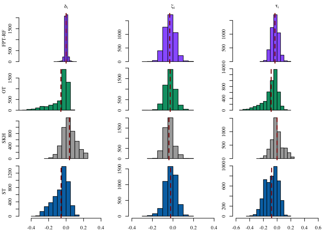
[1,] -0.03169326Let us visualize the distribution on the individuals effects for each transport-based method, in Figure 14.2 (frequency on the y-axis).
Codes to create the Figure.
library(tikzDevice)
source("../scripts/utils.R")
plot_hist_effects <- function(x,
var_name,
tikz = FALSE,
fill = "red",
printed_method = "",
x_lim = NULL,
print_main = TRUE,
print_x_axis = TRUE) {
if (print_main == TRUE) {
name_effect <- case_when(
str_detect(var_name, "^delta_0") ~ "$\\delta_i$",#"$\\delta_i(0)$",
str_detect(var_name, "^zeta_1") ~ "$\\zeta_i$",#"$\\zeta_i(1)$",
str_detect(var_name, "^tot_effect") ~ "$\\tau_i$",#"$\\tau_i(1)$",
TRUE ~ "other"
)
if (tikz == FALSE) name_effect <- latex2exp::TeX(name_effect)
} else {
name_effect <- ""
}
if (var_name == "tot_effect") {
data_plot <- x[["delta_0_i"]] + x[["zeta_1_i"]]
} else {
data_plot <- x[[var_name]]
}
if (is.null(x_lim)) {
hist(
data_plot,
main = "", xlab = "", ylab = "", family = font_family,
col = fill, axes = FALSE
)
} else {
hist(
data_plot,
main = "", xlab = "", ylab = "", family = font_family,
col = fill, xlim = x_lim, axes = FALSE
)
}
if (print_x_axis) axis(1, family = font_family)
axis(2, family = font_family)
title(
main = name_effect, cex.main = 1, family = font_family
)
if (printed_method != "") {
title(
ylab = printed_method, line = 2,
cex.lab = 1, family = font_family
)
}
abline(v = mean(data_plot), col = "darkred", lty = 2, lwd = 2)
}
colour_methods <- c(
"fairadapt_rf" = "#9966FF",
# "OT" = "#CC79A7",
"OT-M" = "#009E73",
"skh" = "darkgray",
"seq_1" = "#0072B2"
#"seq_2" = "#D55E00",
)
export_tikz <- FALSE
scale <- 1.42
file_name <- "compas-dist-indiv-effects"
width_tikz <- 2.25*scale
height_tikz <- 1.4*scale
if (export_tikz == TRUE)
tikz(paste0("figs/", file_name, ".tex"), width = width_tikz, height = height_tikz)
layout(
matrix(1:12, byrow = TRUE, ncol = 3),
widths = c(1, rep(.9, 2)), heights = c(1, rep(.72, 2))
)
for (i in 1:4) {
x <- case_when(
i == 1 ~ causal_effects_fairadapt_rf,
i == 2 ~ causal_effects_ot,
i == 3 ~ causal_effects_sink_ot,
i == 4 ~ causal_effects_st
)
method <- case_when(
i == 1 ~ "FPT-RF",
i == 2 ~ "OT-M",
i == 3 ~ "SKH",
i == 4 ~ "ST",
)
for (var_name in c("delta_0_i", "zeta_1_i", "tot_effect")) {
mar_bottom <- ifelse(i == 4, 2.1, .6)
mar_left <- ifelse(var_name == "delta_0_i", 3.1, 2.1)
mar_top <- ifelse(i == 1, 2.1, .1)
mar_right <- .4
printed_method <- ifelse(
var_name == "delta_0_i",
ifelse(method == "OT-M", "OT", method),
""
)
par(mar = c(mar_bottom, mar_left, mar_top, mar_right))
x_lim_list <- list(
"delta_0_i" = c(-.5, .5),
"zeta_1_i" = c(-.4, .4),
"tot_effect" = c(-.6, .6)
)
plot_hist_effects(
x = x, var_name = var_name, tikz = export_tikz,
fill = colour_methods[i],
printed_method = printed_method,
x_lim = x_lim_list[[var_name]],
print_main = i == 1,
print_x_axis = i == 4
)
}
}
if (export_tikz == TRUE) {
dev.off()
plot_to_pdf(
filename = file_name,
path = "./figs/", keep_tex = FALSE, crop = T
)
}
14.3.6 With Normalizing Flows
We export the dataset to estimate the causal effect using normalizing flows with the python library medflow (see the Github page of medflow). The python script is provided below but is not run during the compilation of this page. Note that this procedure does not provide individual effects, but aggregated ones.
save(tb, file = "../output/compas.rda")
write_csv(tb, file = "../output/compas.csv")import numpy as np
import os
from medflow import train_med, sim_med
import pandas as pd
df2 = pd.read_csv("compas.csv")
df2["c_charge_degree"] = (df2["c_charge_degree"] == "F").astype(int)
df2.to_csv("compas_cleaned.csv", index=False)
base_path = './' # Define the base path for file operations.
folder = '.' # Define the folder where files will be stored.
path = os.path.join(base_path, folder, '') # Combines the base path and folder into a complete path.
dataset_name = 'compas_cleaned' # Define the name of the dataset.
if not (os.path.isdir(path)): # checks if a directory with the name 'path' exists.
os.makedirs(path) # if not, creates a new directory with this name. This is where the logs and model weights will be saved.
## MODEL TRAINING (~25 min)
train_med(path=path,
dataset_name=dataset_name,
treatment='race',
confounder=[],
mediator=["age", "priors_count","c_charge_degree"],
outcome='is_recid',
test_size=0.2,
cat_var=["c_charge_degree"],
sens_corr=None,
seed_split=1,
model_name=path + 'seed_1',
trn_batch_size=64,
val_batch_size=512,
learning_rate=1e-4,
seed=1,
nb_epoch=3000,
nb_estop=20,
val_freq=1,
emb_net=[164, 48, 32],
int_net=[32, 24, 16]
)
## EFFECT ESTIMATION (~3 minutes)
# Path-specific effects
sim_med(
path=path,
dataset_name=dataset_name,
model_name=path + 'seed_1',
n_mce_samples=10000, seed=1,
inv_datafile_name='1_path_100k_v2',
cat_list=[0, 1],
moderator=None
)In this page, we load the results:
nf_estim <- read.csv("../output/1_path_100k_v2_results.csv")We compute the direct, indirect and total effects
nf_tot_effect <-
nf_estim |> filter(Potential.Outcome == "E[is_recid(race=1)]") |> pull("Value") -
nf_estim |> filter(Potential.Outcome == "E[is_recid(race=0)]") |> pull("Value")
# Indirect
nf_delta_0 <-
nf_estim |> filter(
Potential.Outcome == "E[is_recid(race=0, age(race=1), priors_count(race=1), c_charge_degree(race=1))]"
) |> pull("Value") -
nf_estim |> filter(
Potential.Outcome == "E[is_recid(race=0)]"
) |> pull("Value")
# Direct
nf_zeta_1 <- nf_tot_effect - nf_delta_0
# Sanity check for direct effect
nf_estim |> filter(
Potential.Outcome == "E[is_recid(race=1)]"
) |> pull("Value")-
nf_estim |> filter(
Potential.Outcome == "E[is_recid(race=0, age(race=1), priors_count(race=1), c_charge_degree(race=1))]"
) |> pull("Value")[1] -0.000448435514.3.7 Summary
tibble::tribble(
~method, ~delta_0, ~zeta_1, ~tot_effect,
"CM", delta_0_med, zeta_1_med, tot_effect_med,
"FPT-RF", causal_effects_fairadapt_rf$delta_0, causal_effects_fairadapt_rf$zeta_1, causal_effects_fairadapt_rf$tot_effect,
"FPT-LIN", causal_effects_fairadapt_lin$delta_0, causal_effects_fairadapt_lin$zeta_1, causal_effects_fairadapt_lin$tot_effect,
"NF", nf_delta_0, nf_zeta_1, nf_tot_effect,
"OT", causal_effects_ot$delta_0, causal_effects_ot$zeta_1, causal_effects_ot$tot_effect,
"SKH", causal_effects_sink_ot$delta_0, causal_effects_sink_ot$zeta_1, causal_effects_sink_ot$tot_effect,
"ST", causal_effects_st$delta_0, causal_effects_st$zeta_1, causal_effects_st$tot_effect
) |>
knitr::kable(digits = 3)| method | delta_0 | zeta_1 | tot_effect |
|---|---|---|---|
| CM | -0.091 | 0.005 | -0.086 |
| FPT-RF | 0.000 | -0.031 | -0.031 |
| FPT-LIN | 0.000 | -0.032 | -0.032 |
| NF | -0.061 | 0.000 | -0.061 |
| OT | -0.060 | -0.027 | -0.087 |
| SKH | 0.038 | -0.039 | -0.001 |
| ST | -0.057 | -0.023 | -0.080 |
14.3.8 Decomposition of the Indirect Effect
Due to the iterative nature of the sequential transport approach, which follows the topological order of the mediators in the causal graph, it is possible to further decompose the causal influence of each mediator on the indirect effect at the individual level.
# Load sequential_transport
load("../output/seq-t-compas.rda")Total indirect effect with the Sequential Transport approach:
causal_effects_st$delta_0[1] -0.05742751Before decomposing the indirect effect, we need to retrieve the fitted RF model of the total indirect effect.
# Observations
data_untreated <- tb_untreated
# All variables transported
data_cf_untreated <- as_tibble(sequential_transport$transported)

Y_name <- Y_name
A_name <- A_name

# Outcome model for untreated
mu_untreated_model <- randomForest(
  x = data_untreated |> dplyr::select(-!!Y_name, -!!A_name),
  y = pull(data_untreated, !!Y_name)
)
Now we can modify the causal_effects_cf() to take the fitted RF model as an argument to be able to decompose the indirect effect and we return only the indirect effect at the individual level, delta_0_i and the average delta_0.
modified_causal_effects_cf <- function(data_untreated,
                                       data_cf_untreated,
                                       mu_untreated_model) {

  n_untreated <- nrow(data_untreated)

  # Natural Indirect Effect, using predictions
  delta_0_i <- predict(mu_untreated_model, newdata = data_cf_untreated) -
      predict(mu_untreated_model, newdata = data_untreated)
  delta_0 <- mean(delta_0_i)

  list(
    delta_0_i = delta_0_i,
    delta_0 = delta_0
  )
}
The total indirect effect is:
modified_causal_effects_cf(data_untreated, data_cf_untreated, mu_untreated_model)$delta_0[1] -0.0560891514.3.8.1 Influence of Age
cf_treated_first <- data_untreated |>
  mutate(age = as_tibble(sequential_transport$transported)$age)

indirect_age <- modified_causal_effects_cf(
  data_untreated = data_untreated,
  data_cf_untreated = cf_treated_first,
  mu_untreated_model = mu_untreated_model
)

cbind(
  delta_0_age = indirect_age$delta_0
)
delta_0_age
[1,] -0.0346605814.3.8.2 Influence of Prior Counts
cf_treated_second <- cf_treated_first |>
  mutate(priors_count = as_tibble(sequential_transport$transported)$priors_count)

indirect_priors_count <- modified_causal_effects_cf(
  data_untreated = cf_treated_first,
  data_cf_untreated = cf_treated_second,
  mu_untreated_model = mu_untreated_model
)

cbind(
  delta_0_priors_count = indirect_priors_count$delta_0
)
delta_0_priors_count
[1,] -0.0175071214.3.8.3 Influence of Charge Degree
cf_treated_third <- cf_treated_second |>
  mutate(c_charge_degree = as_tibble(sequential_transport$transported)$c_charge_degree)

indirect_c_charge_degree <- modified_causal_effects_cf(
  data_untreated = cf_treated_second,
  data_cf_untreated = cf_treated_third,
  mu_untreated_model = mu_untreated_model
)

cbind(
  delta_0_c_charge_degree = indirect_c_charge_degree$delta_0
)
delta_0_c_charge_degree
[1,] -0.00392145