11  Small Example

Objectives

In the previous chapters, we explored how to construct counterfactuals for a categorical variable by mapping individuals from one group (group 0) to another (group 1). We considered three approaches: random matching (Chapter 11), optimal transport based on arbitrarily assigned numerical values to the categories (Chapter 9), and optimal transport using a representation in the probability simplex (Chapter 10). In this chapter, we illustrate these methods on a small example involving six individuals in each group, and compare the resulting counterfactual assignments for the categorical variable.

Codes for graphical parameters
# col_categ <- c("#ffdd55","#944edf","#3fb3b2")
col_group <- c("#00A08A","#F2AD00", "#1b95e0")
col_categ <- c("#56B4E9", "#D55E00", "#CC79A7")
colA <- col_categ[1] ; colB <- col_categ[2] ; colC <- col_categ[3]
colGpe1 <- col_group[2]
colGpe0 <- col_group[1]
font_size <- 20
font_family <- "CMU Serif"

path <- "./figs/"

theme_ggtern_paper <- function(...) {
  font_family <- "CMU Serif"
  font_size <- 10
  theme(
    strip.background = element_rect(colour = "black", fill = NA),
    strip.text.x = element_text(colour = "black"),
    strip.text = ggtext::element_markdown(),
    text = element_text(family = font_family, size = unit(font_size, "pt")),
    axis.title = element_text(size = rel(1)),
    tern.axis.arrow.show = TRUE,
    tern.axis.arrow.sep = .13,
    tern.axis.vshift = .05,
    panel.border = element_rect(colour = NA)
  )
}

theme_ggtern <- function(...) {
  font_family <- "CMU Serif"
  font_size <- 20
  theme(
    strip.background = element_rect(colour = "black", fill = NA),
    strip.text.x = element_text(colour = "black"),
    strip.text = ggtext::element_markdown(),
    text = element_text(family = font_family, size = unit(font_size, "pt")),
    axis.title = element_text(size = rel(1)),
    tern.axis.arrow.show = TRUE,
    tern.axis.arrow.sep = .13,
    tern.axis.vshift = .05,
    panel.border = element_rect(colour = NA)
  )
}

theme_ggtern_minimal <- function(...) {
  font_family <- "CMU Serif"
  font_size <- 10
  theme(
    strip.background = element_rect(colour = "black", fill = NA),
    # strip.text.x = element_text(colour = "black"),
    # strip.text = ggtext::element_markdown(),
    text = element_text(family = font_family, size = unit(font_size, "pt")),
    axis.title = element_text(size = rel(1)),
    tern.axis.arrow.show = FALSE,
    tern.axis.arrow.sep = .13,
    tern.axis.vshift = .05,
    panel.border = element_rect(colour = NA),
    tern.axis.text.T = element_blank(),
    tern.axis.text.L = element_blank(),
    tern.axis.text.R = element_blank(),
    tern.axis.vshift = 0.2
  )
}


#' Theme for ggplot2
#'
#' @param ... Arguments passed to the theme function.
#' @export
#' @importFrom ggplot2 element_rect element_text element_blank element_line unit
#'   rel theme
#'
theme_paper <- function (...) {
  theme(
    text = element_text(family = font_family),
    plot.background = element_rect(fill = "transparent", color = NA),
    panel.background = element_rect(fill = "transparent", color = NA),
    # panel.border = element_rect(fill = NA, colour = "black", linewidth = 1),
    panel.border = element_blank(),
    # axis.line = element_line(color = "black"),
    axis.line <- element_blank(),
    axis.text = element_text(color = "black"),
    legend.text = element_text(size = rel(1)),
    legend.title = element_text(size = rel(1)),
    legend.background = element_rect(fill = "transparent", color = NULL),
    # legend.position = "bottom",
    # legend.direction = "horizontal",
    # legend.box = "vertical",
    legend.key = element_blank(),
    panel.spacing = unit(1, "lines"),
    panel.grid.major = element_line(colour = "grey90"),
    panel.grid.minor = element_blank(),
    plot.title = element_text(hjust = 0, size = rel(1), face = "bold"),
    plot.title.position = "plot",
    plot.margin = unit(c(1, 1, 1, 1), "lines"),
    strip.background = element_rect(fill = NA, colour = NA),
    strip.text = element_text(size = rel(1))
  )
}

\[ \definecolor{wongBlack}{RGB}{0,0,0} \definecolor{wongGold}{RGB}{230, 159, 0} \definecolor{wongLightBlue}{RGB}{86, 180, 233} \definecolor{wongGreen}{RGB}{0, 158, 115} \definecolor{wongYellow}{RGB}{240, 228, 66} \definecolor{wongBlue}{RGB}{0, 114, 178} \definecolor{wongOrange}{RGB}{213, 94, 0} \definecolor{wongPurple}{RGB}{204, 121, 167} %\definecolor{colA}{RGB}{255, 221, 85} %\definecolor{colB}{RGB}{148, 78, 223} %\definecolor{colC}{RGB}{63, 179, 178} \definecolor{colA}{RGB}{0, 114, 178} \definecolor{colB}{RGB}{213, 94, 0} \definecolor{colC}{RGB}{204, 121, 167} \definecolor{colGpeZero}{RGB}{0,160,138} \definecolor{colGpeUn}{RGB}{242, 173, 0} \]

library(dplyr)
library(tidyr)
library(stringr)
library(ggtern)
library(compositions)
library(clue)

Let us consider a simplistic toy example.

As in the previous chapters, assume two groups: 0 and 1. In the first group, there are \(n_0=6\) individuals indexed 1, 2, 3, 4, 5, 6; and in group 1, there are \(n_1=6\) individuals indexed 7, 8, 9, 10, 11, 12. Let \(Y\) denote a response variable that takes values in \(\mathbb{R}\), and let \(X\) be a categorical variable taking values \(\{A,B,C\}\).

Let us assume that we obtained the estimated probabilities of being in each class using a multinomial regression model. This allows to convert categorical observations \(\{x_{1,1},\cdots,x_{1,n_1}\}\) and \(\{x_{0,1},\cdots,x_{0,n_0}\}\) into estimated probabilities, \(\{\boldsymbol{p}_{1,1},\cdots,\boldsymbol{p}_{1,n_1}\}\) and \(\{\boldsymbol{p}_{0,1},\cdots,\boldsymbol{p}_{0,n_0}\}\).

Let us create a toy example:

group_0 <- tribble(
  ~i, ~x, ~p_A, ~p_B, ~p_C, ~y,
  1, "A", .8,   .1,   .1,   1,
  2, "A", .7,   .2,   .1,   2,
  3, "A", .6,   .1,   .3,   3,
  4, "B", .2,   .7,   .1,   4,
  5, "B", .3,   .6,   .1,   5,
  6, "C", .1,   .2,   .7,   6
)

group_1 <- tribble(
  ~i, ~x, ~p_A, ~p_B, ~p_C, ~y,
  7,  "A", .7,  .2,   .1,   3,
  8,  "B", .1,  .7,   .2,   4,
  9,  "B", .6,  .2,   .2,   5,
  10, "B", .2,  .5,   .3,   6,
  11, "C", .3,  .1,   .6,   7,
  12, "C", .1,  .3,   .6,   8
)

11.1 Random Matching

There are \(6!=720\) different random matching that can be done. We will show two of them below.

11.1.1 First Random Matching

Let us first consider a random matching in which the individuals matched are 1 (group 0) and 12 (group 1), 2 and 9, 3 and 7, 4 and 10, 5 and 8, 6 and 12.

matched_ex_1 <- tribble(
  ~i_0, ~i_1,
  1, 12,
  2, 9,
  3, 7,
  4, 10,
  5, 8,
  6, 11
) |>
  left_join(
    group_0 |>
      rename_with(~str_c(.x, "_0")),
    by = "i_0"
  ) |>
  left_join(
    group_1 |>
      rename_with(~str_c(.x, "_1")),
    by = "i_1"
  )

11.1.2 Second Random Matching

We can consider, for the sake of illustration, a second random matching, where the individuals matched are 1 and 8, 2 and 7, 3 and 11, 4 and 10, 5 and 9, 6 and 12.

matched_ex_2 <- tribble(
  ~i_0, ~i_1,
  1, 8,
  2, 7,
  3, 11,
  4, 10,
  5, 9,
  6, 12
) |>
  left_join(
    group_0 |>
      rename_with(~str_c(.x, "_0")),
    by = "i_0"
  ) |>
  left_join(
    group_1 |>
      rename_with(~str_c(.x, "_1")),
    by = "i_1"
  )

11.2 Matching on Arbitrarily Assigned Numerical Values to the Categories

Let us arbitrarily set the following values for the categories: \(A=1\), \(B=2\), \(C=3\).

cat_levels <- c("A", "B", "C")
x0_index <- match(group_0$x, cat_levels)
x1_index <- match(group_1$x, cat_levels)

For the cost matrix, we can use the Euclidean distance between the arbitrarily assigned numerical values.

cost_matrix <- outer(x0_index, x1_index, function(i, j) sqrt((i - j)^2))
cost_matrix
     [,1] [,2] [,3] [,4] [,5] [,6]
[1,]    0    1    1    1    2    2
[2,]    0    1    1    1    2    2
[3,]    0    1    1    1    2    2
[4,]    1    0    0    0    1    1
[5,]    1    0    0    0    1    1
[6,]    2    1    1    1    0    0

Using this cost matrix, the transport problem can be solved with the solve_LSAP() function from {clue}.

assignment <- solve_LSAP(cost_matrix)

We add the IDs of each observation:

n0 <- nrow(group_0)
n1 <- nrow(group_1)
ot_plan_num <- tibble(
  from = 1:n0,
  to = as.numeric(assignment)
)
ot_plan_num$i_0 <- group_0$i[ot_plan_num$from]
ot_plan_num$i_1 <- group_1$i[ot_plan_num$to]
ot_plan_num
# A tibble: 6 × 4
   from    to   i_0   i_1
  <int> <dbl> <dbl> <dbl>
1     1     1     1     7
2     2     4     2    10
3     3     6     3    12
4     4     2     4     8
5     5     3     5     9
6     6     5     6    11

The matched individuals are shown in Figure 11.2.

Codes to create the Figure.
ggtern(
  data = group_0 |> mutate(group = "0") |> 
    bind_rows(group_1 |> mutate(group = "1")) |> 
    left_join(
      ot_plan_num |> 
        mutate(
          id_match = as.character(row_number())
        ) |> 
        dplyr::select(i_0, i_1, id_match) |> 
        pivot_longer(cols = c(i_0, i_1), values_to = "i") |> 
        dplyr::select(-name),
      by = "i"
    ),
  mapping = aes(x = p_A, y = p_B, z = p_C, group = id_match)
) +
  geom_point(mapping = aes(shape = group, colour = x), size = 4) +
  geom_text(
    mapping = aes(
      label = i, 
      x = p_A + ifelse(group == 0, -1, 1) * 0.05
    ),
    size = .3*font_size
  ) +
  labs(x = "$p_A$", y = "$p_B$", z = "$p_C") +
  geom_line(
    colour = "gray40", 
    # mapping = aes(linetype = id_match)
  ) +
  scale_colour_manual(
    name = "category", 
    values = col_categ, 
    labels = c("A" = "A=1", "B" = "B=2", "C" = "C=3")
  ) +
  scale_shape_discrete(name = "group") +
  theme_light(base_size = font_size, base_family = font_family) +
  # theme_paper() +
  theme_ggtern() +
  theme(
    legend.title = element_text(size = .8*font_size),
    legend.text = element_text(size = .8*font_size)
  ) +
  theme_latex(TRUE) +
  theme_hidetitles()
Figure 11.1: 1-to-1 Matching with optimal transport based on the distances between the individuals with respect to the abrbitrarily assigned numerical values to the categories.

11.3 Transport on Simplex

Let us now perform optimal matching between individuals from the two groups with optimal transport using a representation in the probability simplex.s

11.3.1 Matching Using the Euclidean Distances Cost Matrix

Let us use the Euclidean distance for the transport costs. These distances are computed in the space of centered log-ratio (clr) transformed probability vectors associated with each individual’s membership in one of the classes.

Let us first extract the probability vectors (\(p_A, p_B, p_C\)) from both groups and apply the clr transformation to make them suitable for Euclidean geometry in the compositional space.

library(compositions)
all_coords <- rbind(
  as.matrix(group_0[, c("p_A", "p_B", "p_C")]),
  as.matrix(group_1[, c("p_A", "p_B", "p_C")])
) |> 
  clr()

Then, we can compute the pairwise Euclidean distances between individuals in group 0 and those in group 1, based on their clr-transformed probability vectors.

row.names(all_coords) <- c(group_0$i, group_1$i)
# Euclidean distances between the clr transform of the propensities
D <- as.matrix(dist(all_coords, method = "euclidean"))
n0 <- nrow(group_0)
n1 <- nrow(group_1)
between_distances <- D[1:n0, (n0 + 1):(n0 + n1)]
round(between_distances, 2)
     7    8    9   10   11   12
1 0.63 2.91 0.80 2.27 1.99 2.92
2 0.00 2.42 0.64 1.85 2.09 2.67
3 1.30 2.67 0.79 1.93 0.98 2.21
4 1.77 0.98 1.78 1.06 2.67 2.09
5 1.38 1.30 1.46 1.15 2.53 2.21
6 2.75 1.77 2.16 1.36 1.30 0.41

We aim to find the optimal matching between the individuals in group 1 and group 0 based on these distances. Formally, we want to solve the following optimal transport problem: \[ \min_{P\in\mathcal{U}(\boldsymbol{1}_{n_1},\boldsymbol{1}_{n_0})} \langle P,\,C\rangle, \] where \(C:=[C_{i,j}]\) is the cost matrix, with \(C_{ij}\) measuring the cost of matching individual \(i\) from group 1 to individual \(j\) from group 0. Here, we use the Euclidean distance that we juste computed. The total cost is given by \(\langle P, C\rangle=\sum_{i=1}^{n_1}\sum_{j=1}^{n_0}P_{ij}\,C_{ij}\). The set of admissible transport plans is defined as follows: \[ \left\{\,P\in\mathbb{R}_+^{n_1\times n_0}: P\,\mathbf{1}_{n_0}=\frac{\mathbf{1}_{n_1}}{n_1},\ P^\top\mathbf{1}_{n_1}=\frac{\mathbf{1}_{n_0}}{n_0} \right\}. \] We thus have a uniform mass distribution across both groups.

Note

An alternative cost function (which is not used here) is the cross-entropy between two compositional vectors: \[ \begin{equation*} c(\mathbf{x},\mathbf{y})=\log\left(\frac{1}{d}\sum_{i=1}^d\frac{y_i}{x_i}\right)-\frac{1}{d}\sum_{i=1}^d\log\left(\frac{y_i}{x_i}\right), \end{equation*}. \] This corresponds to the “Dirichlet transport” (Baxendale and Wong (2022)). This alternative is considered below, in Section 11.3.2.

We solve the optimal transport problem using the transport() function from the {transport} package. This function computes the optimal matching plan based on the cost matrix.

# source weights
mass_source <- rep(1 / n0, n0)
# target weights
mass_target <- rep(1 / n1, n1)

# Solve the optimal transport plan
ot_plan <- transport::transport(
  a = mass_source, b = mass_target, costm = between_distances, 
  method = "networkflow"
)
ot_plan$i_0 <- group_0$i[ot_plan$from]
ot_plan$i_1 <- group_1$i[ot_plan$to]
ot_plan
  from to      mass i_0 i_1
1    1  3 0.1666667   1   9
2    2  1 0.1666667   2   7
3    3  5 0.1666667   3  11
4    4  2 0.1666667   4   8
5    5  4 0.1666667   5  10
6    6  6 0.1666667   6  12

We can visualize the results in a ternary plot (Figure 11.2). The lines depict the matched individuals (shown by dots and their index).

Codes to create the Figure.
all_data <- group_0 |> mutate(group = "0") |> 
  bind_rows(group_1 |> mutate(group = "1"))

library(ggtern)

p <- ggtern(
  data = all_data |> 
    left_join(
      ot_plan |> 
        mutate(
          i_0 = as.numeric(i_0),
          i_1 = as.numeric(i_1),
          id_match = as.character(row_number())
        ) |> 
        dplyr::select(i_0, i_1, id_match) |> 
        pivot_longer(cols = c(i_0, i_1), values_to = "i") |> 
        dplyr::select(-name)
    ),
  mapping = aes(x = p_A, y = p_B, z = p_C, group = id_match)
) +
  geom_point(mapping = aes(shape = group, colour = x), size = 4) +
  geom_text(
    mapping = aes(
      label = i, 
      x = p_A + ifelse(group == 0, -1, 1) * 0.05
    ),
    size = .3*font_size
  ) +
  labs(x = "$p_A$", y = "$p_B$", z = "$p_C") +
  geom_line(
    colour = "gray40", 
    # mapping = aes(linetype = id_match)
  ) +
  scale_colour_manual(name = "category", values = col_categ) +
  scale_shape_discrete(name = "group") +
  theme_light(base_size = font_size, base_family = font_family) +
  # theme_paper() +
  theme_ggtern() +
  theme(
    legend.title = element_text(size = .8*font_size),
    legend.text = element_text(size = .8*font_size)
  ) +
  theme_latex(TRUE) +
  theme_hidetitles()

p
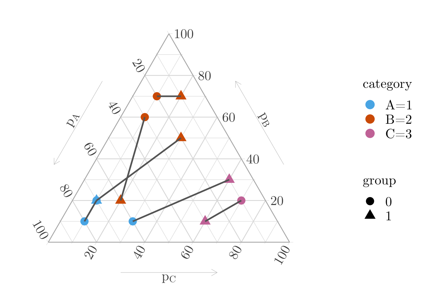
Figure 11.2: 1-to-1 Matching with optimal transport based on the distances between the individuals with respect to their estimated probabilities of being in each class.
Codes to export the figure in PDF.
filename <- "ternary-toy"
ggsave(
  p, file = str_c(path, filename, ".pdf"),
  height = 2.2*1.75, width = 4*1.75,
  family = font_family,
  device = cairo_pdf
)
Warning: Removing Layer 2 ('PositionNudge'), as it is not an approved position
(for ternary plots) under the present ggtern package.
Codes to export the figure in PDF.
# Crop PDF
system(paste0("pdfcrop ", path, filename, ".pdf ", path, filename, ".pdf"))

11.3.2 Matching Using the Cross-Entropy Cost Matrix

In Section 11.3.1, we used the Euclidean distance of the clr-transformed vector of probabilities as the cost function to solve the optimal transport problem. Here, we consider an alternative cost function, the cross-entreopy: \[ c(\mathbf{x}, \mathbf{y}) = \log\left(\frac{1}{d} \sum_{i=1}^d \frac{y_i}{x_i}\right) - \frac{1}{d} \sum_{i=1}^d \log\left(\frac{y_i}{x_i}\right). \]

We first extract the probability vectors for the individuals from both groups (without clr transform), and we make sure there is no probability equal to 0.

p0 <- as.matrix(group_0[, c("p_A", "p_B", "p_C")])
p1 <- as.matrix(group_1[, c("p_A", "p_B", "p_C")])
p0 <- pmax(p0, 1e-10)
p1 <- pmax(p1, 1e-10)

Let us define the cross-entropy cost function:

cross_entropy_cost <- function(x, y) {
  d <- length(x)
  log(mean(y / x)) - mean(log(y / x))
}

We can then compute the pairwise cost matrix (group0 rows vs group1 columns).

between_distances_ce <- outer(
  1:nrow(p0), 1:nrow(p1),
  Vectorize(function(i, j) cross_entropy_cost(p0[i, ], p1[j, ]))
)
round(between_distances_ce, 4)
       [,1]   [,2]   [,3]   [,4]   [,5]   [,6]
[1,] 0.0694 0.9259 0.0933 0.5710 0.6292 0.8421
[2,] 0.0000 0.6318 0.0716 0.4027 0.7533 0.8514
[3,] 0.2379 1.0435 0.1048 0.5769 0.1542 0.5436
[4,] 0.4670 0.1542 0.3867 0.1979 0.8514 0.7533
[5,] 0.2844 0.2379 0.2718 0.2352 0.8708 0.8232
[6,] 0.9985 0.4670 0.7076 0.2424 0.2894 0.0287

Then, we can solde the optimal transport problem.

ot_plan_ce <- transport::transport(
  a = mass_source,
  b = mass_target,
  costm = between_distances_ce,
  method = "networkflow"
)
ot_plan_ce$i_0 <- group_0$i[ot_plan_ce$from]
ot_plan_ce$i_1 <- group_1$i[ot_plan_ce$to]
ot_plan_ce
  from to      mass i_0 i_1
1    1  3 0.1666667   1   9
2    2  1 0.1666667   2   7
3    3  5 0.1666667   3  11
4    4  2 0.1666667   4   8
5    5  4 0.1666667   5  10
6    6  6 0.1666667   6  12

Again, we can visualize the matched individuals on a ternary plot (Figure 11.3).

Codes to create the Figure.
ggtern(
  data = all_data |> 
    left_join(
      ot_plan_ce |> 
        mutate(
          i_0 = as.numeric(i_0),
          i_1 = as.numeric(i_1),
          id_match = as.character(row_number())
        ) |> 
        dplyr::select(i_0, i_1, id_match) |> 
        pivot_longer(cols = c(i_0, i_1), values_to = "i") |> 
        dplyr::select(-name)
    ),
  mapping = aes(x = p_A, y = p_B, z = p_C, group = id_match)
) +
  geom_point(mapping = aes(shape = group, colour = x), size = 4) +
  geom_text(
    mapping = aes(
      label = i, 
      x = p_A + ifelse(group == 0, -1, 1) * 0.05
    ),
    size = .3*font_size
  ) +
  labs(x = "$p_A$", y = "$p_B$", z = "$p_C") +
  geom_line(
    colour = "gray40", 
    # mapping = aes(linetype = id_match)
  ) +
  scale_colour_manual(name = "category", values = col_categ) +
  scale_shape_discrete(name = "group") +
  theme_light(base_size = font_size, base_family = font_family) +
  # theme_paper() +
  theme_ggtern() +
  theme(
    legend.title = element_text(size = .8*font_size),
    legend.text = element_text(size = .8*font_size)
  ) +
  theme_latex(TRUE) +
  theme_hidetitles()
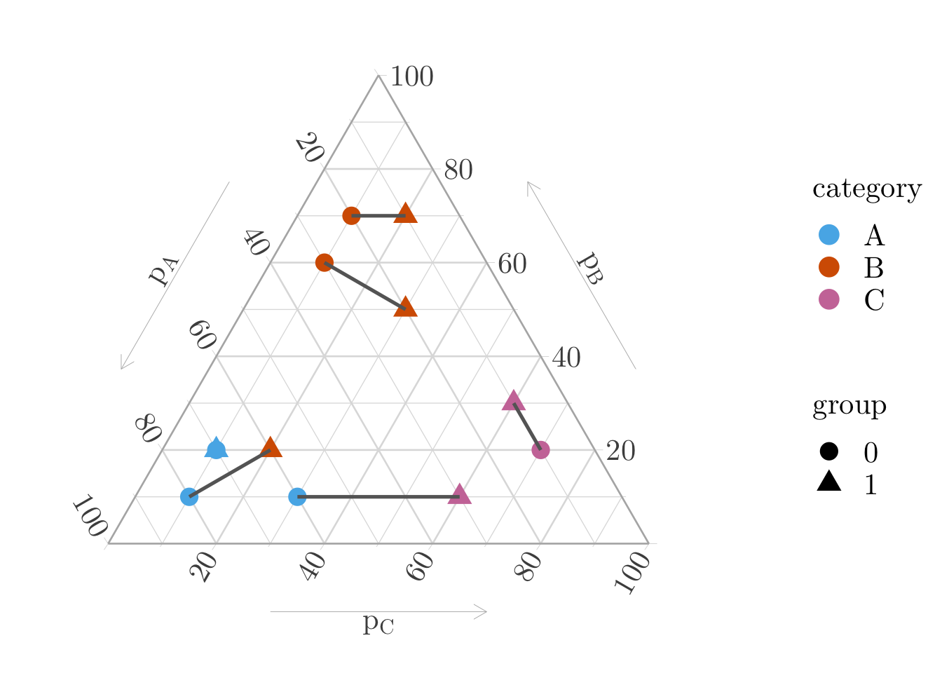
Figure 11.3: 1-to-1 Matching with optimal transport based on cross entropy as the transport cost between the individuals with respect to their estimated probabilities of being in each class.