This chapter investigates how the distribution of estimated scores by an extreme gradient boosting model evolves with the number of boosting iterations. In the models we train, we vary the maximum depth of trees and consider boosting iterations up to 400. For each configuration, we compute the predicted scores from iteration 1 to 400; for each boosting iteration, we use the predicted scores (both on train set and on test set) to compute various metrics (performance, calibration, divergence between the distribution of scores and that of true underlying probabilities).
library(tidyverse)
── Attaching core tidyverse packages ──────────────────────── tidyverse 2.0.0 ──
✔ dplyr     1.1.4     ✔ readr     2.1.5
✔ forcats   1.0.0     ✔ stringr   1.5.1
✔ ggplot2   3.5.1     ✔ tibble    3.2.1
✔ lubridate 1.9.3     ✔ tidyr     1.3.1
✔ purrr     1.0.2
── Conflicts ────────────────────────────────────────── tidyverse_conflicts() ──
✖ dplyr::filter() masks stats::filter()
✖ dplyr::lag()    masks stats::lag()
ℹ Use the conflicted package (<http://conflicted.r-lib.org/>) to force all conflicts to become errors
library(ggh4x)
Attaching package: 'ggh4x'

The following object is masked from 'package:ggplot2':

    guide_axis_logticks
library(ggrepel)library(rpart)library(locfit)
locfit 1.5-9.9   2024-03-01

Attaching package: 'locfit'

The following object is masked from 'package:purrr':

    none
library(philentropy)# Colours for train/validation/testcolour_samples <-c("Train"="#0072B2","Validation"="#009E73","Test"="#D55E00")
definition of the theme_paper() function (for ggplot2 graphs)
We generate data using the first 12 scenarios from Ojeda et al. (2023) and an additional set of 4 scenarios in which the true probability does not depend on the predictors in a linear way (see Chapter 4).
When we simulate a dataset, we draw the following number of observations:
nb_obs <-10000
Definition of the 16 scenarios
# Coefficients betacoefficients <-list(# First category (baseline, 2 covariates)c(0.5, 1), # scenario 1, 0 noise variablec(0.5, 1), # scenario 2, 10 noise variablesc(0.5, 1), # scenario 3, 50 noise variablesc(0.5, 1), # scenario 4, 100 noise variables# Second category (same as baseline, with lower number of 1s)c(0.5, 1), # scenario 5, 0 noise variablec(0.5, 1), # scenario 6, 10 noise variablesc(0.5, 1), # scenario 7, 50 noise variablesc(0.5, 1), # scenario 8, 100 noise variables# Third category (same as baseline but with 5 num. and 5 categ. covariates)c(0.1, 0.2, 0.3, 0.4, 0.5, 0.01, 0.02, 0.03, 0.04, 0.05),c(0.1, 0.2, 0.3, 0.4, 0.5, 0.01, 0.02, 0.03, 0.04, 0.05),c(0.1, 0.2, 0.3, 0.4, 0.5, 0.01, 0.02, 0.03, 0.04, 0.05),c(0.1, 0.2, 0.3, 0.4, 0.5, 0.01, 0.02, 0.03, 0.04, 0.05),# Fourth category (nonlinear predictor, 3 covariates)c(0.5, 1, .3), # scenario 5, 0 noise variablec(0.5, 1, .3), # scenario 6, 10 noise variablesc(0.5, 1, .3), # scenario 7, 50 noise variablesc(0.5, 1, .3) # scenario 8, 100 noise variables)# Mean parameter for the normal distribution to draw from to draw num covariatesmean_num <-list(# First category (baseline, 2 covariates)rep(0, 2), # scenario 1, 0 noise variablerep(0, 2), # scenario 2, 10 noise variablesrep(0, 2), # scenario 3, 50 noise variablesrep(0, 2), # scenario 4, 100 noise variables# Second category (same as baseline, with lower number of 1s)rep(0, 2), # scenario 5, 0 noise variablerep(0, 2), # scenario 6, 10 noise variablesrep(0, 2), # scenario 7, 50 noise variablesrep(0, 2), # scenario 8, 100 noise variables# Third category (same as baseline but with 5 num. and 5 categ. covariates)rep(0, 5),rep(0, 5),rep(0, 5),rep(0, 5),# Fourth category (nonlinear predictor, 3 covariates)rep(0, 3),rep(0, 3),rep(0, 3),rep(0, 3))# Sd parameter for the normal distribution to draw from to draw num covariatessd_num <-list(# First category (baseline, 2 covariates)rep(1, 2), # scenario 1, 0 noise variablerep(1, 2), # scenario 2, 10 noise variablesrep(1, 2), # scenario 3, 50 noise variablesrep(1, 2), # scenario 4, 100 noise variables# Second category (same as baseline, with lower number of 1s)rep(1, 2), # scenario 5, 0 noise variablerep(1, 2), # scenario 6, 10 noise variablesrep(1, 2), # scenario 7, 50 noise variablesrep(1, 2), # scenario 8, 100 noise variables# Third category (same as baseline but with 5 num. and 5 categ. covariates)rep(1, 5),rep(1, 5),rep(1, 5),rep(1, 5),# Fourth category (nonlinear predictor, 3 covariates)rep(1, 3),rep(1, 3),rep(1, 3),rep(1, 3))params_df <-tibble(scenario =1:16,coefficients = coefficients,n_num =c(rep(2, 8), rep(5, 4), rep(3, 4)),add_categ =c(rep(FALSE, 8), rep(TRUE, 4), rep(FALSE, 4)),n_noise =rep(c(0, 10, 50, 100), 4),mean_num = mean_num,sd_num = sd_num,size_train =rep(nb_obs, 16),size_valid =rep(nb_obs, 16),size_test =rep(nb_obs, 16),transform_probs =c(rep(FALSE, 4), rep(TRUE, 4), rep(FALSE, 4), rep(FALSE, 4)),linear_predictor =c(rep(TRUE, 12), rep(FALSE, 4)),seed =202105)rm(coefficients, mean_num, sd_num)
8.2 Metrics
We load the functions from Chapter 3 to compute performance, calibration and divergence metrics.
source("functions/metrics.R")
8.3 Simulations Setup
To train the models, we rely on the {xgboost} R package.
library(xgboost)
Attaching package: 'xgboost'
The following object is masked from 'package:dplyr':

    slice
As explained in the foreword of this page, we compute metrics based on scores obtained at various boosting iterations. To do so, we define a function, get_metrics_nb_iter(), that will be applied to a fitted model. This function will be called for all the boosting iterations (controlled by the nb_iter argument). The function returns a list with the following elements:
scenario: the ID of the scenario
ind: the index of the grid search (so that we can join with the hyperparameters values, if needed)
repn: the ID of the replication
nb_iter: the boosting iteration at which the metrics are computed
tb_metrics: the tibble with the performance, calibration, and divergence metrics (one row for the train sample, one row for the validation sample, and one row for the test sample)
tb_prop_scores: additional metrics (\(\mathbb{P}(q_1 < \hat{s}(\mathbf{x}) < q_2)\) for multiple values for \(q_1\) and \(q_2 = 1-q_1\))
scores_hist: elements to be able to plot an histogram of the scores on both the train set and the test set (using 20 equally-sized bins over \([0,1]\)).
Function get_metrics_nb_iter()
#' Computes the performance and calibration metrics for an xgb model,#' depending on the number of iterations kept.#'#' @param nb_iter number of boosting iterations to keep#' @param params hyperparameters of the current model#' @param fitted_xgb xgb estimated model#' @param tb_train_xgb train data (in xgb.DMatrix format)#' @param tb_valid_xgb validation data (in xgb.DMatrix format)#' @param tb_test_xgb test data (in xgb.DMatrix format)#' @param simu_data simulated dataset#' @param true_prob list with true probabilities on train, validation and#' test setsget_metrics_nb_iter <-function(nb_iter, params, fitted_xgb, tb_train_xgb, tb_valid_xgb, tb_test_xgb, simu_data, true_prob) { ind <- params$ind max_depth <- params$max_depth tb_train <- simu_data$data$train |>rename(d = y) tb_valid <- simu_data$data$valid |>rename(d = y) tb_test <- simu_data$data$test |>rename(d = y)# Predicted scores scores_train <-predict(fitted_xgb, tb_train_xgb, iterationrange =c(1, nb_iter)) scores_valid <-predict(fitted_xgb, tb_valid_xgb, iterationrange =c(1, nb_iter)) scores_test <-predict(fitted_xgb, tb_test_xgb, iterationrange =c(1, nb_iter))## Histogram of scores---- breaks <-seq(0, 1, by = .05) scores_train_hist <-hist(scores_train, breaks = breaks, plot =FALSE) scores_valid_hist <-hist(scores_valid, breaks = breaks, plot =FALSE) scores_test_hist <-hist(scores_test, breaks = breaks, plot =FALSE) scores_hist <-list(train = scores_train_hist,valid = scores_valid_hist,test = scores_test_hist,scenario = simu_data$scenario,ind = ind,repn = simu_data$repn,max_depth = params$max_depth,nb_iter = nb_iter )## Estimation of P(q1 < score < q2)---- proq_scores_train <-map(c(.1, .2, .3, .4),~prop_btw_quantiles(s = scores_train, q1 = .x) ) |>list_rbind() |>mutate(sample ="train") proq_scores_valid <-map(c(.1, .2, .3, .4),~prop_btw_quantiles(s = scores_valid, q1 = .x) ) |>list_rbind() |>mutate(sample ="valid") proq_scores_test <-map(c(.1, .2, .3, .4),~prop_btw_quantiles(s = scores_test, q1 = .x) ) |>list_rbind() |>mutate(sample ="test")## Dispersion Metrics---- disp_train <-dispersion_metrics(true_probas = true_prob$train, scores = scores_train ) |>mutate(sample ="train") disp_valid <-dispersion_metrics(true_probas = true_prob$valid, scores = scores_valid ) |>mutate(sample ="valid") disp_test <-dispersion_metrics(true_probas = true_prob$test, scores = scores_test ) |>mutate(sample ="test")# Performance and Calibration Metrics# We add very small noise to predicted scores# otherwise the local regression may crash scores_train_noise <- scores_train +runif(n =length(scores_train), min =0, max =0.01) scores_train_noise[scores_train_noise >1] <-1 metrics_train <-compute_metrics(obs = tb_train$d, scores = scores_train_noise, true_probas = true_prob$train ) |>mutate(sample ="train") scores_valid_noise <- scores_valid +runif(n =length(scores_valid), min =0, max =0.01) scores_valid_noise[scores_valid_noise >1] <-1 metrics_valid <-compute_metrics(obs = tb_valid$d, scores = scores_valid_noise, true_probas = true_prob$valid ) |>mutate(sample ="valid") scores_test_noise <- scores_test +runif(n =length(scores_test), min =0, max =0.01) scores_test_noise[scores_test_noise >1] <-1 metrics_test <-compute_metrics(obs = tb_test$d, scores = scores_test_noise, true_probas = true_prob$test ) |>mutate(sample ="test") tb_metrics <- metrics_train |>bind_rows(metrics_valid) |>bind_rows(metrics_test) |>left_join( disp_train |>bind_rows(disp_valid) |>bind_rows(disp_test),by ="sample" ) |>mutate(scenario = simu_data$scenario,ind = ind,repn = simu_data$repn,max_depth = params$max_depth,# type = !!type,nb_iter = nb_iter ) tb_prop_scores <- proq_scores_train |>bind_rows(proq_scores_valid) |>bind_rows(proq_scores_test) |>mutate(scenario = simu_data$scenario,ind = ind,repn = simu_data$repn,max_depth = params$max_depth,nb_iter = nb_iter )list(scenario = simu_data$scenario, # data scenarioind = ind, # index for gridrepn = simu_data$repn, # data replication IDnb_iter = nb_iter, # number of boosting iterationstb_metrics = tb_metrics, # table with performance/calib/divergence# metricstb_prop_scores = tb_prop_scores, # table with P(q1 < score < q2)scores_hist = scores_hist # histogram of scores )}
We define another function, simul_xgb() which trains an extreme gradient boosting model for a single replication. It calls the get_metrics_nb_iter() on each of the boosting iterations of the model from the second to the last (400th), and returns a list of length 400-1 where each element is a list returned by the get_metrics_nb_iter().
Function simul_xgb()
#' Train an xgboost model and compute performance, calibration, and dispersion#' metrics#'#' @param params tibble with hyperparameters for the simulation#' @param ind index of the grid (numerical ID)#' @param simu_data simulated data obtained with `simulate_data_wrapper()`simul_xgb <-function(params, ind, simu_data) { tb_train <- simu_data$data$train |>rename(d = y) tb_valid <- simu_data$data$valid |>rename(d = y) tb_test <- simu_data$data$test |>rename(d = y) true_prob <-list(train = simu_data$data$probs_train,valid = simu_data$data$probs_valid,test = simu_data$data$probs_test )## Format data for xgboost---- tb_train_xgb <-xgb.DMatrix(data =model.matrix(d ~-1+ ., tb_train), label = tb_train$d ) tb_valid_xgb <-xgb.DMatrix(data =model.matrix(d ~-1+ ., tb_valid), label = tb_valid$d ) tb_test_xgb <-xgb.DMatrix(data =model.matrix(d ~-1+ ., tb_test), label = tb_test$d )# Parameters for the algorithm param <-list(max_depth = params$max_depth, #Note: root node is indexed 0eta = params$eta,nthread =1,objective ="binary:logistic",eval_metric ="auc" ) watchlist <-list(train = tb_train_xgb, eval = tb_valid_xgb)## Estimation---- xgb_fit <-xgb.train( param, tb_train_xgb,nrounds = params$nb_iter_total, watchlist,verbose =0 )# Number of leaves# dt_tree <- xgb.model.dt.tree(model = xgb_fit)# path_depths <- xgboost:::get.leaf.depth(dt_tree)# path_depths |> count(Tree) |> select(n) |> table()# Then, for each boosting iteration number up to params$nb_iter_total# compute the predicted scores and evaluate the metrics resul <-map(seq(2, params$nb_iter_total),~get_metrics_nb_iter(nb_iter = .x,params = params,fitted_xgb = xgb_fit,tb_train_xgb = tb_train_xgb,tb_valid_xgb = tb_valid_xgb,tb_test_xgb = tb_test_xgb,simu_data = simu_data,true_prob = true_prob ), ) resul}simulate_xgb_scenario <-function(scenario, params_df, repn) {# Generate Data simu_data <-simulate_data_wrapper(scenario = scenario,params_df = params_df,repn = repn )# Looping over the grid hyperparameters for the scenario res_simul <-vector(mode ="list", length =nrow(grid)) cli::cli_progress_bar("Iteration grid", total =nrow(grid), type ="tasks")for (j in1:nrow(grid)) { curent_params <- grid |> dplyr::slice(!!j) res_simul[[j]] <-simul_xgb(params = curent_params,ind = curent_params$ind,simu_data = simu_data ) cli::cli_progress_update() }# The metrics computed for all set of hyperparameters (identified with `ind`)# and for each number of boosting iterations (`nb_iter`), for the current# scenario (`scenario`) and current replication number (`repn`) metrics_simul <-map( res_simul,function(simul_grid_j) map(simul_grid_j, "tb_metrics") |>list_rbind() ) |>list_rbind()# Sanity check# metrics_simul |> count(scenario, repn, ind, sample, nb_iter) |># filter(n > 1)# P(q_1<s(x)<q_2) prop_scores_simul <-map( res_simul,function(simul_grid_j) map(simul_grid_j, "tb_prop_scores") |>list_rbind() ) |>list_rbind()# Sanity check# prop_scores_simul |> count(scenario, repn, ind, sample, nb_iter)# Histogram of estimated scores scores_hist <-map( res_simul,function(simul_grid_j) map(simul_grid_j, "scores_hist") )list(metrics_simul = metrics_simul,scores_hist = scores_hist,prop_scores_simul = prop_scores_simul )}
The desired number of replications for each scenario needs to be set:
repns_vector <-1:100
The different configurations are reported in Table 8.1.
DT::datatable(grid)
Table 8.1: Grid Search Values
We define a function, simulate_xgb_scenario() to train the model on a dataset for all different values of the hyperparameters of the grid. This function performs a single replication of the simulations for a single scenario.
Function simulate_xgb_scenario()
simulate_xgb_scenario <-function(scenario, params_df, repn) {# Generate Data simu_data <-simulate_data_wrapper(scenario = scenario,params_df = params_df,repn = repn )# Looping over the grid hyperparameters for the scenario res_simul <-vector(mode ="list", length =nrow(grid)) cli::cli_progress_bar("Iteration grid", total =nrow(grid), type ="tasks")for (j in1:nrow(grid)) { curent_params <- grid |> dplyr::slice(!!j) res_simul[[j]] <-simul_xgb(params = curent_params,ind = curent_params$ind,simu_data = simu_data ) cli::cli_progress_update() }# The metrics computed for all set of hyperparameters (identified with `ind`)# and for each number of boosting iterations (`nb_iter`), for the current# scenario (`scenario`) and current replication number (`repn`) metrics_simul <-map( res_simul,function(simul_grid_j) map(simul_grid_j, "tb_metrics") |>list_rbind() ) |>list_rbind()# Sanity check# metrics_simul |> count(scenario, repn, ind, sample, nb_iter) |># filter(n > 1)# P(q_1<s(x)<q_2) prop_scores_simul <-map( res_simul,function(simul_grid_j) map(simul_grid_j, "tb_prop_scores") |>list_rbind() ) |>list_rbind()# Sanity check# prop_scores_simul |> count(scenario, repn, ind, sample, nb_iter)# Histogram of estimated scores scores_hist <-map( res_simul,function(simul_grid_j) map(simul_grid_j, "scores_hist") )list(metrics_simul = metrics_simul,scores_hist = scores_hist,prop_scores_simul = prop_scores_simul )}
8.4 Estimations
We loop over the 16 scenarios and run the 100 replications in parallel.
The resul_rf object is of length 16: each element contains the simulations for a scenario. For each scenario, the elements are a list of length max(repns_vector), i.e., the number of replications. Each replication gives, in a list, the following elements:
metrics_simul: the metrics (AUC, Calibration, KL Divergence, etc.) for each model from the grid search, for all boosting iterations
scores_hist: the counts on bins defined on estimated scores (on train, validation, and test sets)
prop_scores_simul: the estimations of \(\mathbb{P}(q_1 < \hat{\mathbf{x}}< q_2)\) for various values of q_1 and q_2.
8.5 Results
We can now extract some information from the results.
We first aggregate all the computed metrics performance/calibration/divergence in a single tibble, metrics_xgb_all.
For each replication, we made some hyperparameters vary. Let us identify some models of interest:
smallest: model with the lowest number of boosting iteration
largest: model with the highest number of boosting iteration
largest_auc: model with the highest AUC on validation set
lowest_mse: model with the lowest MSE on validation set
lowest_ici: model with the lowest ICI on validation set
lowest_kl: model with the lowest KL Divergence on validation set
Code
# Identify the model with the smallest number of boosting iterationssmallest_xgb <- metrics_xgb_all |>filter(sample =="Validation") |>group_by(scenario, repn) |>arrange(nb_iter) |>slice_head(n =1) |>select(scenario, repn, ind, nb_iter) |>mutate(result_type ="smallest") |>ungroup()# Identify the largest treelargest_xgb <- metrics_xgb_all |>filter(sample =="Validation") |>group_by(scenario, repn) |>arrange(desc(nb_iter)) |>slice_head(n =1) |>select(scenario, repn, ind, nb_iter) |>mutate(result_type ="largest") |>ungroup()# Identify tree with highest AUC on test sethighest_auc_xgb <- metrics_xgb_all |>filter(sample =="Validation") |>group_by(scenario, repn) |>arrange(desc(AUC)) |>slice_head(n =1) |>select(scenario, repn, ind, nb_iter) |>mutate(result_type ="largest_auc") |>ungroup()# Identify tree with lowest MSElowest_mse_xgb <- metrics_xgb_all |>filter(sample =="Validation") |>group_by(scenario, repn) |>arrange(mse) |>slice_head(n =1) |>select(scenario, repn, ind, nb_iter) |>mutate(result_type ="lowest_mse") |>ungroup()# Identify tree with lowest brierlowest_brier_xgb <- metrics_xgb_all |>filter(sample =="Validation") |>group_by(scenario, repn) |>arrange(brier) |>slice_head(n =1) |>select(scenario, repn, ind, nb_iter) |>mutate(result_type ="lowest_brier") |>ungroup()# Identify tree with lowest ICIlowest_ici_xgb <- metrics_xgb_all |>filter(sample =="Validation") |>group_by(scenario, repn) |>arrange(ici) |>slice_head(n =1) |>select(scenario, repn, ind, nb_iter) |>mutate(result_type ="lowest_ici") |>ungroup()# Identify tree with lowest KLlowest_kl_xgb <- metrics_xgb_all |>filter(sample =="Validation") |>group_by(scenario, repn) |>arrange(KL_20_true_probas) |>slice_head(n =1) |>select(scenario, repn, ind, nb_iter) |>mutate(result_type ="lowest_kl") |>ungroup()# Merge thesemodels_of_interest_xgb <- smallest_xgb |>bind_rows(largest_xgb) |>bind_rows(highest_auc_xgb) |>bind_rows(lowest_mse_xgb) |>bind_rows(lowest_brier_xgb) |>bind_rows(lowest_ici_xgb) |>bind_rows(lowest_kl_xgb)# Add metrics nowmodels_of_interest_metrics <- models_of_interest_xgb |>left_join( metrics_xgb_all,by =c("scenario", "repn", "ind", "nb_iter"),relationship ="many-to-many"# (train, valid, test) )# Sanity check# models_of_interest_metrics |> count(scenario, sample, result_type)
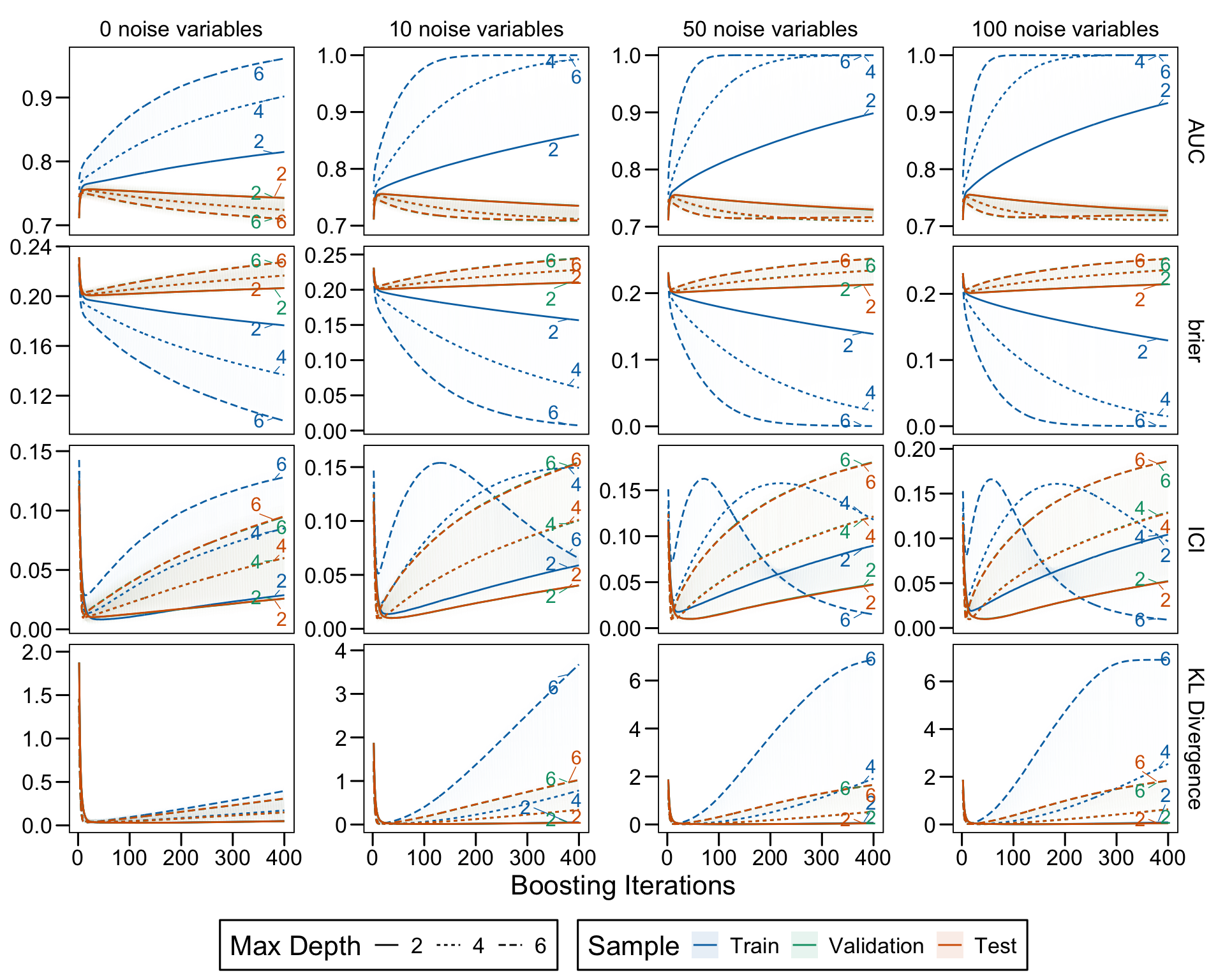
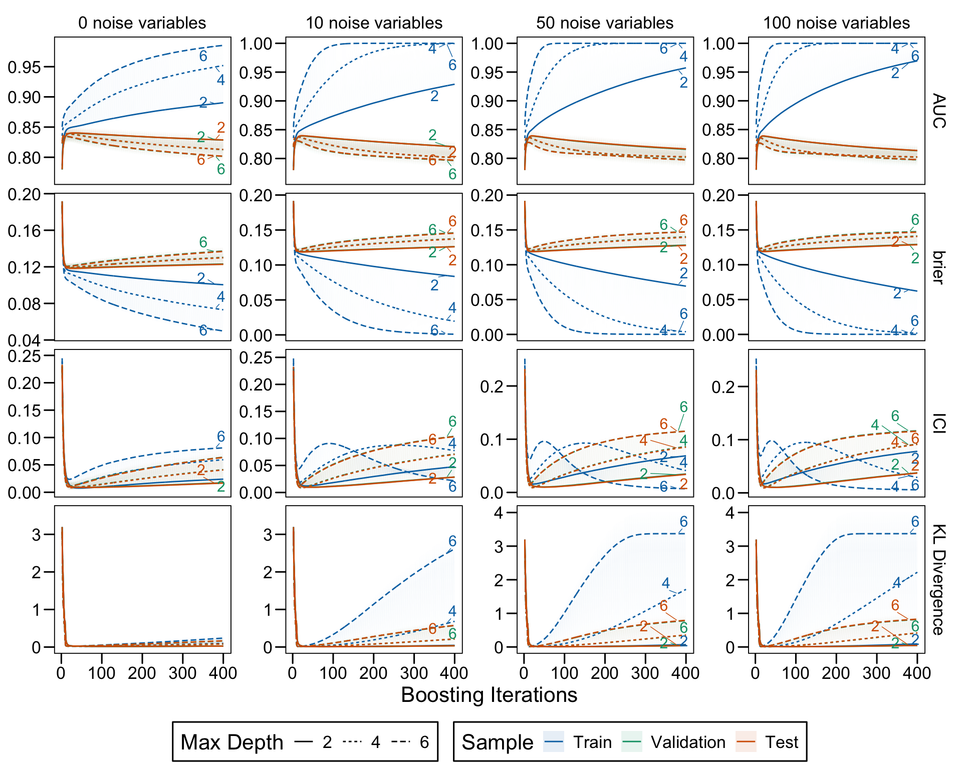
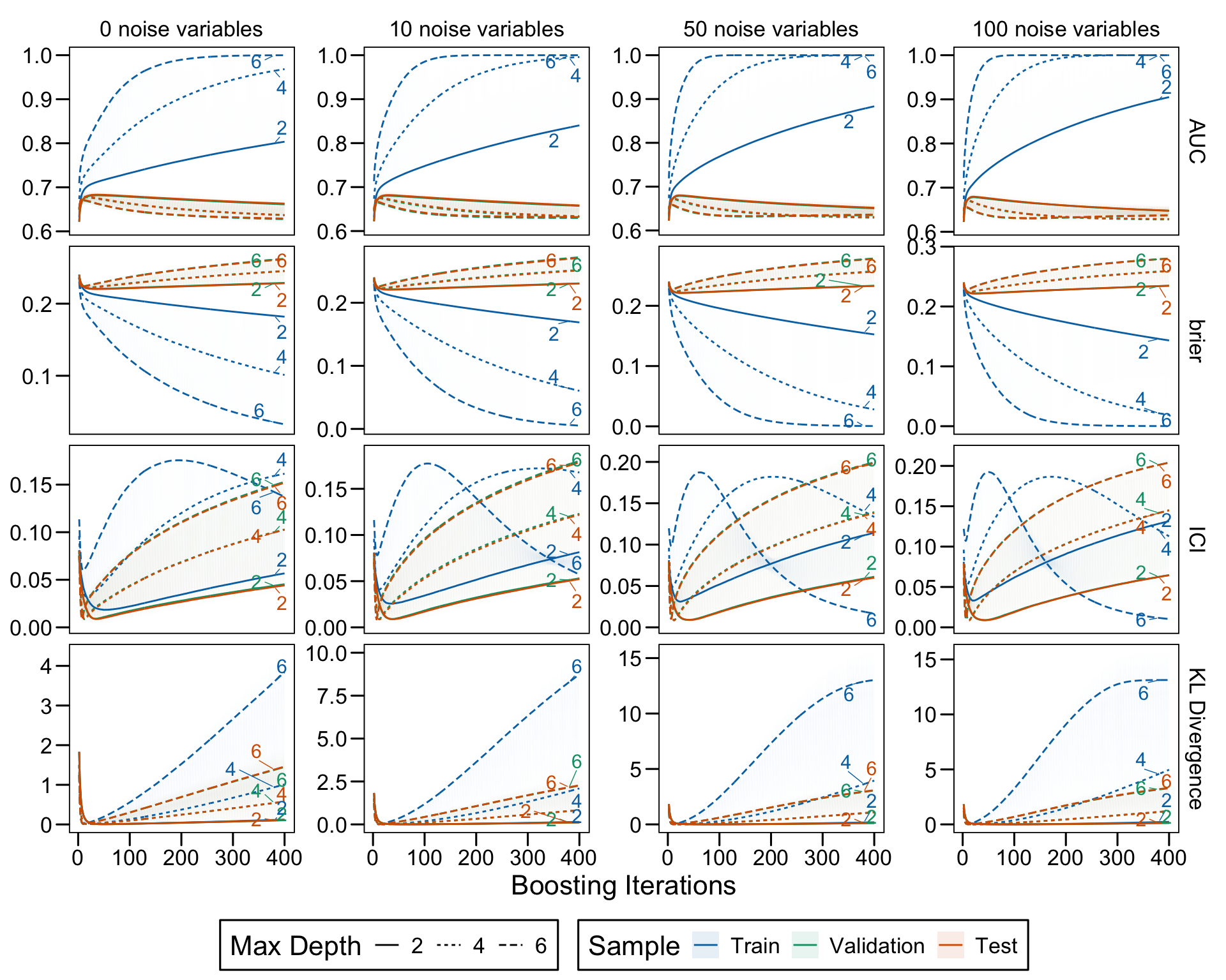
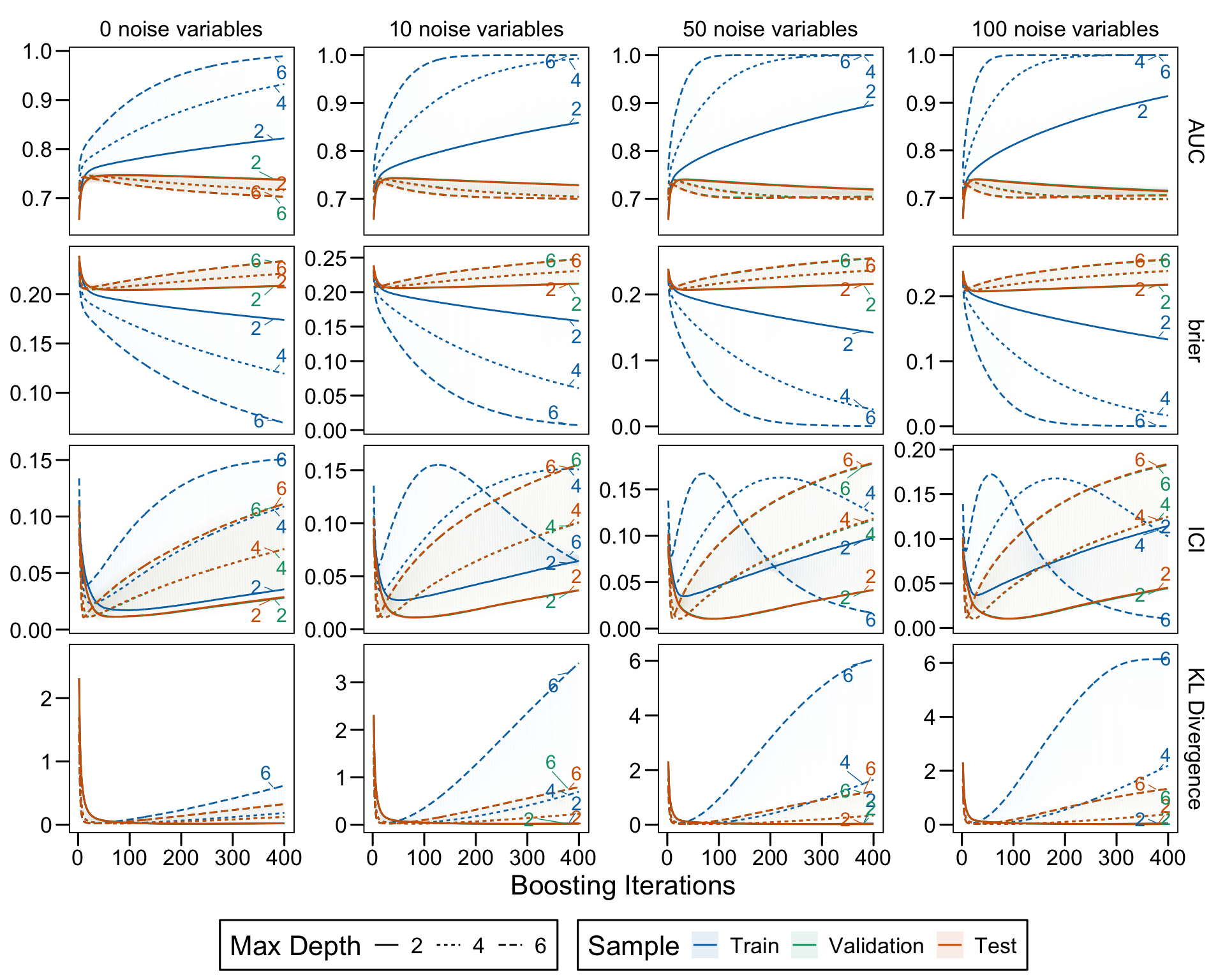
8.5.1 Metrics vs Number of Iterations
We define a function, plot_metrics() to plot selected metrics (AUC, ICI, and KL Divergence) as a function of the number of boosting iterations. Each curve corresponds to a value of the maximal depth hyperparameter.
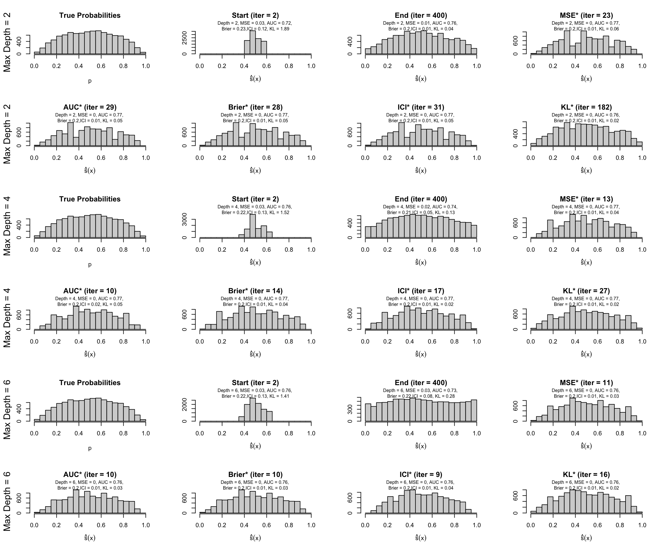
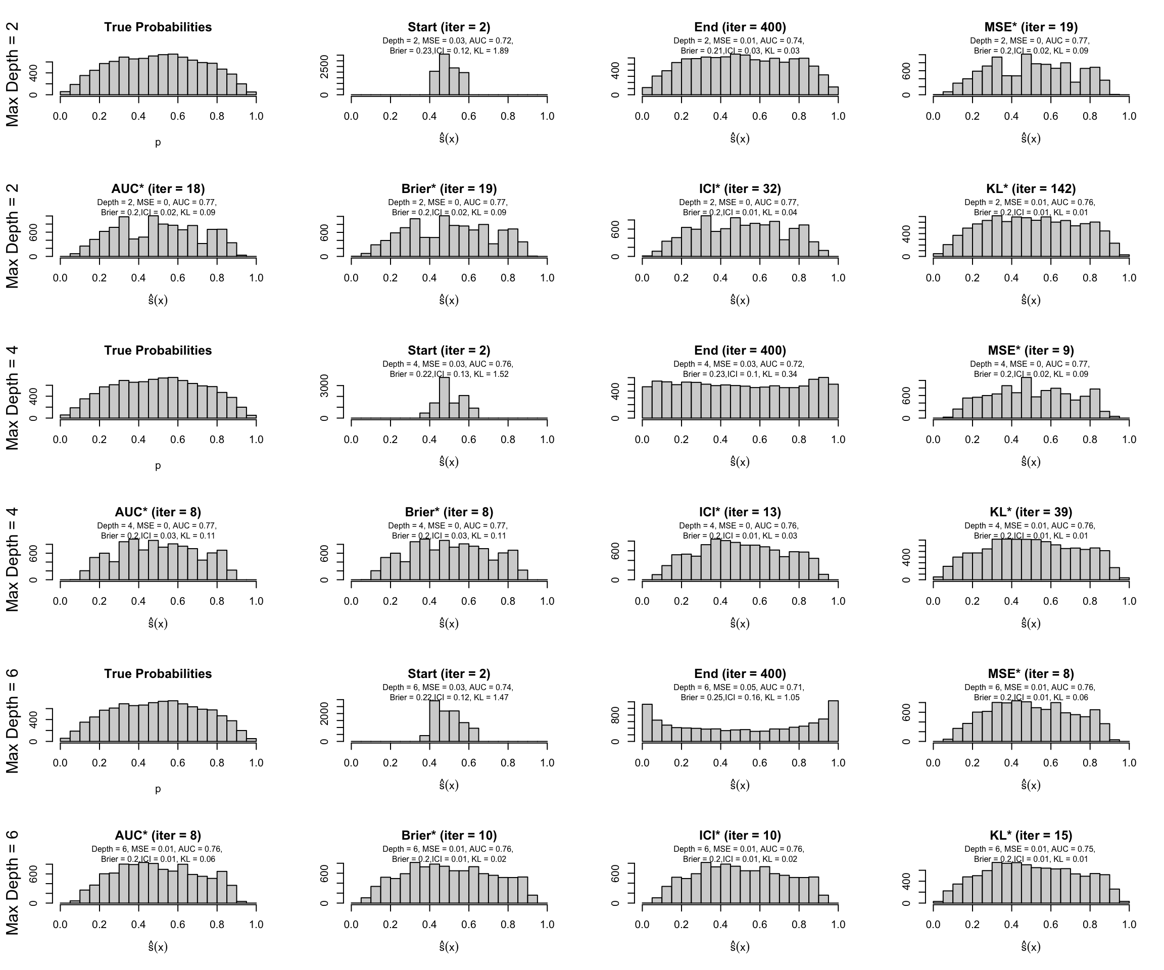
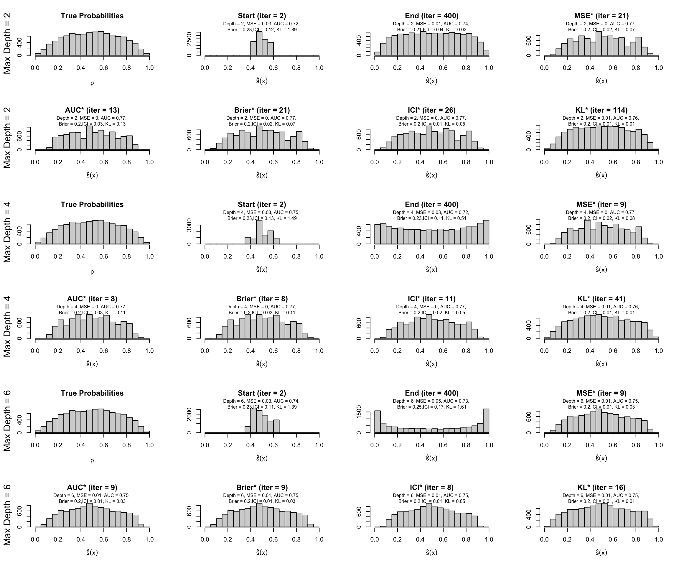
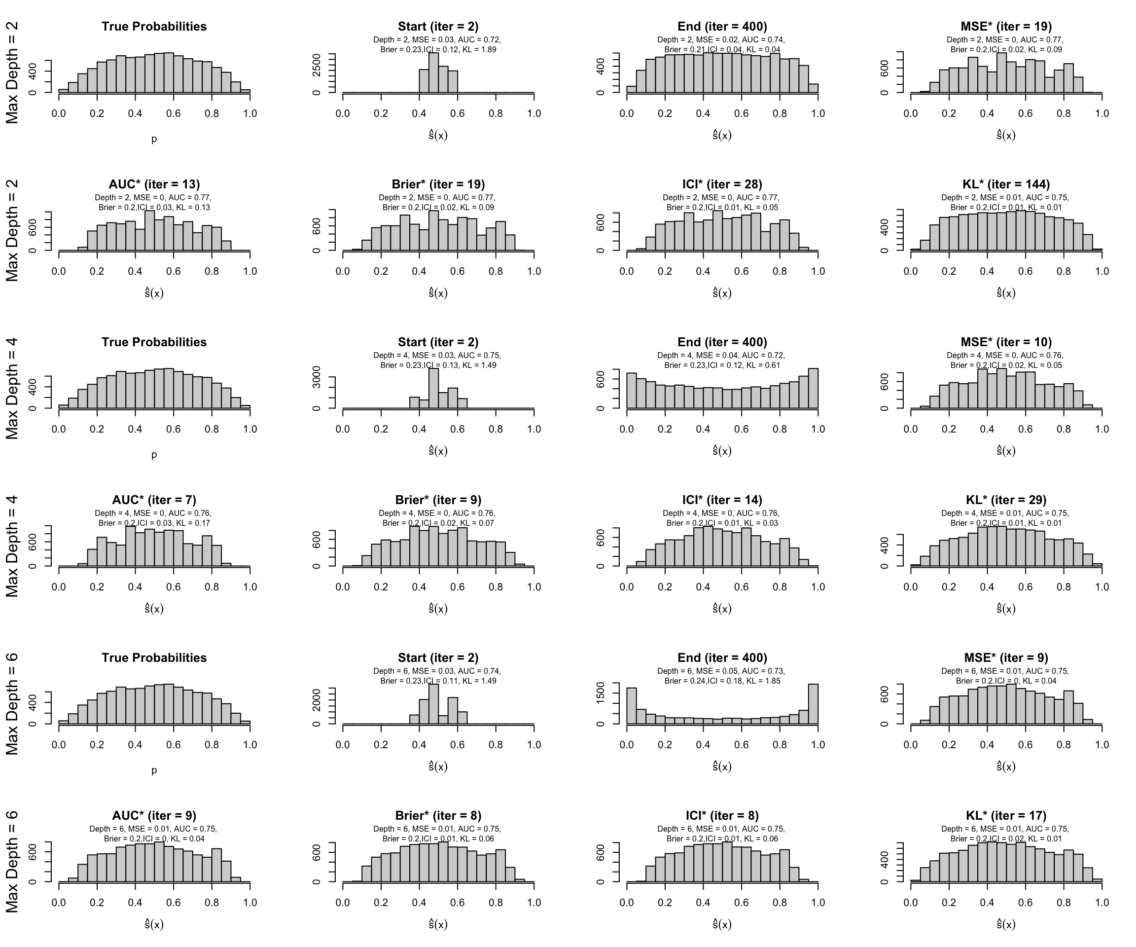
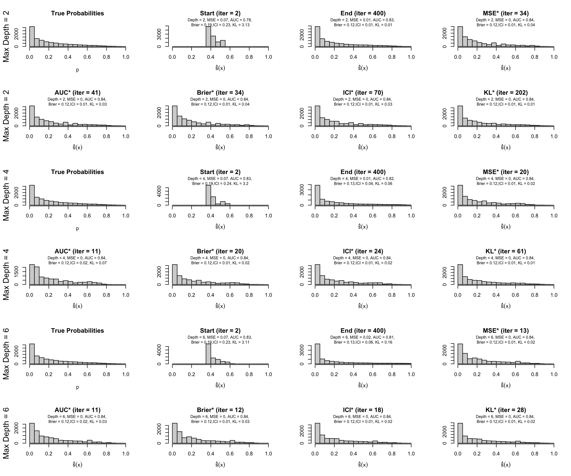
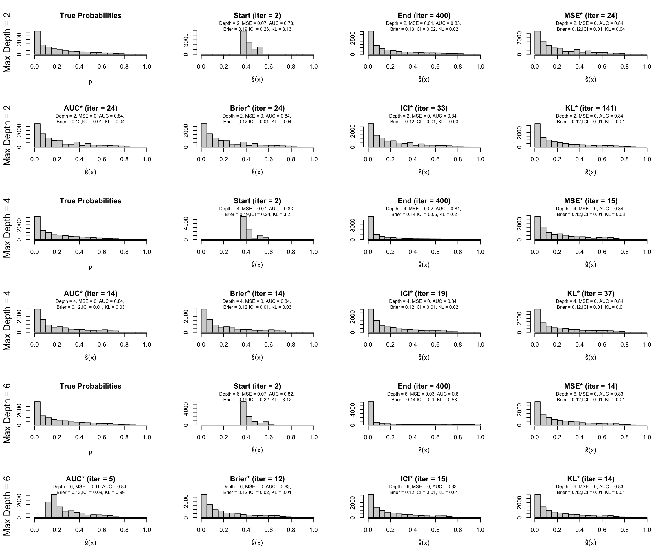
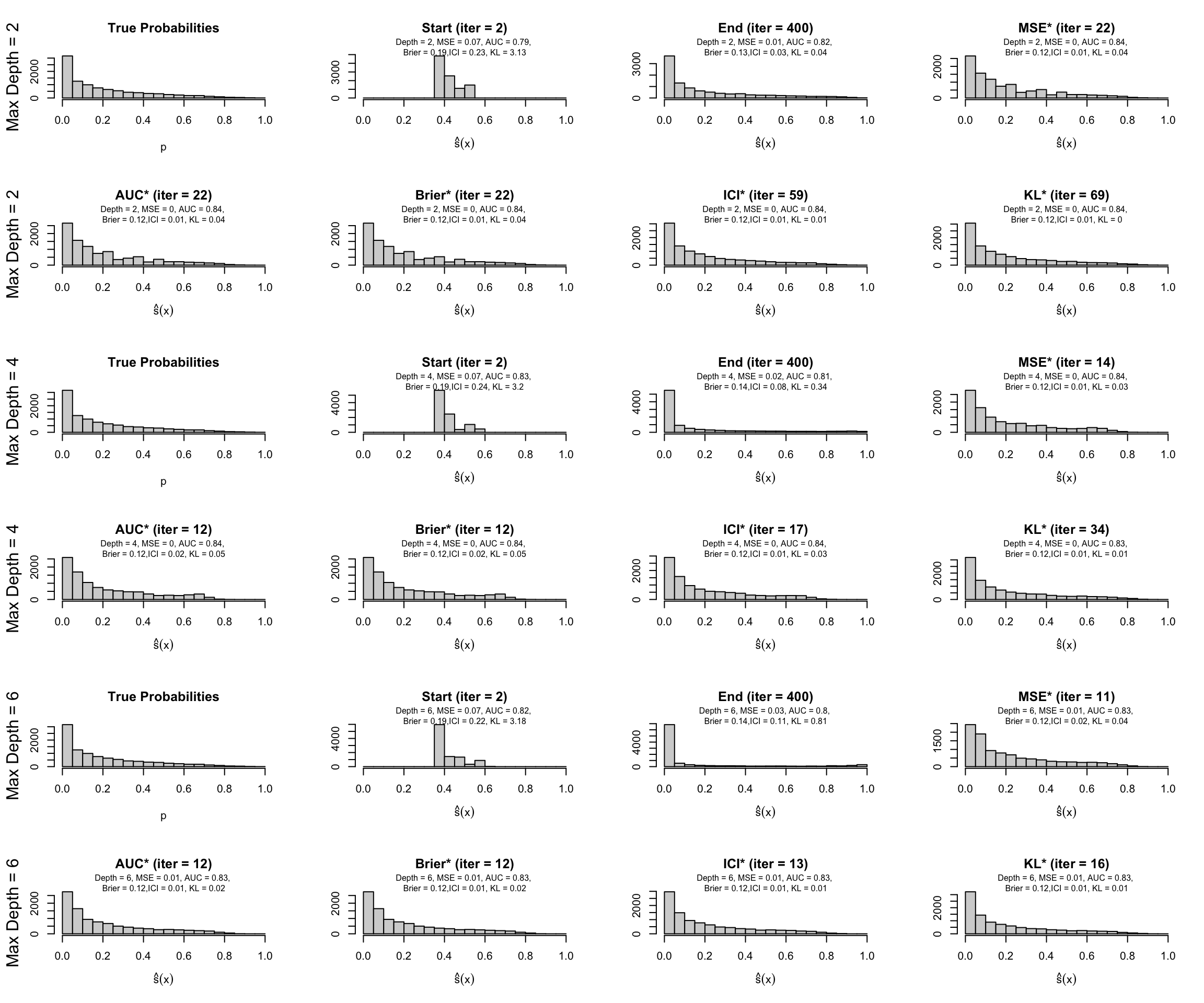
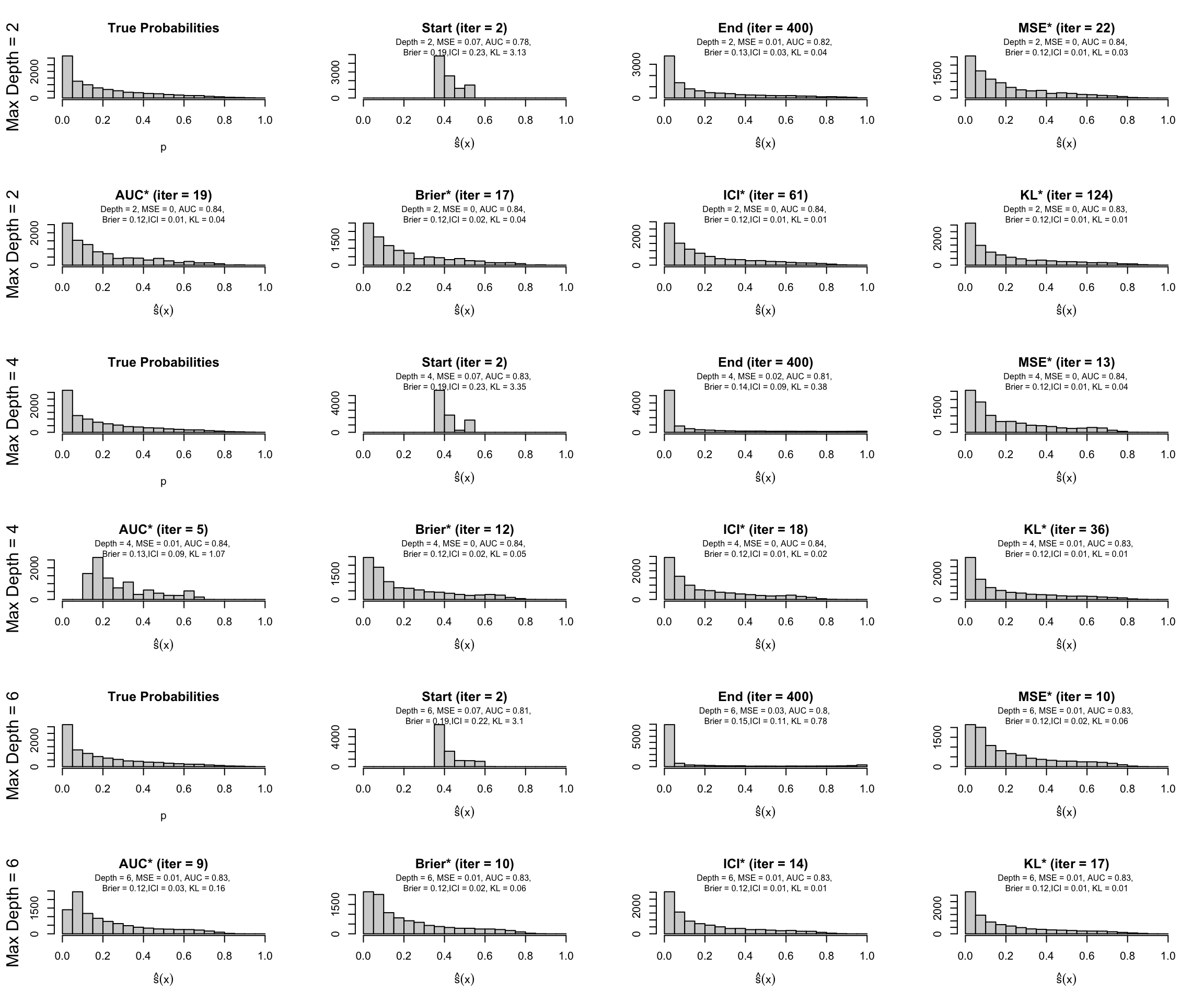
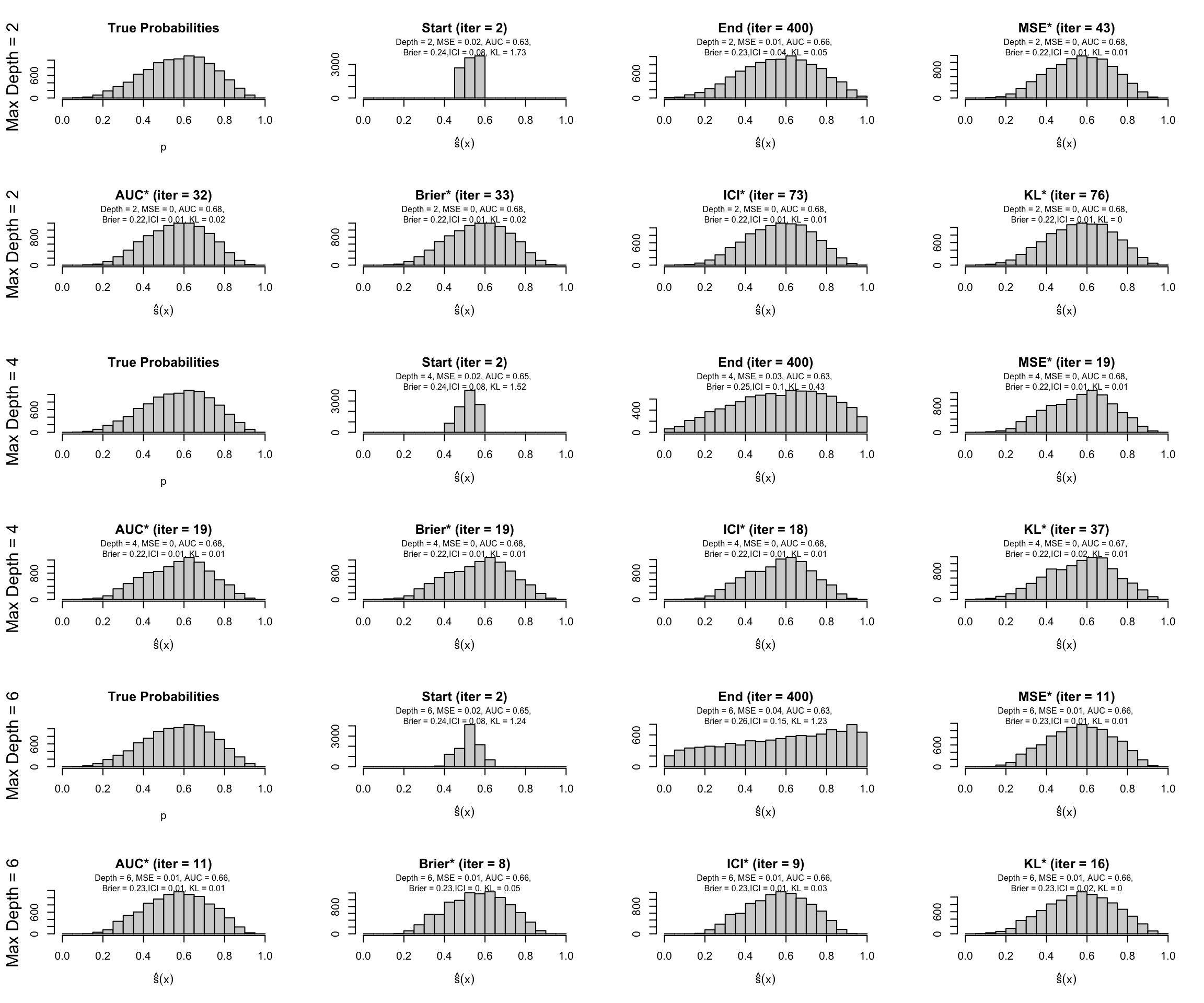
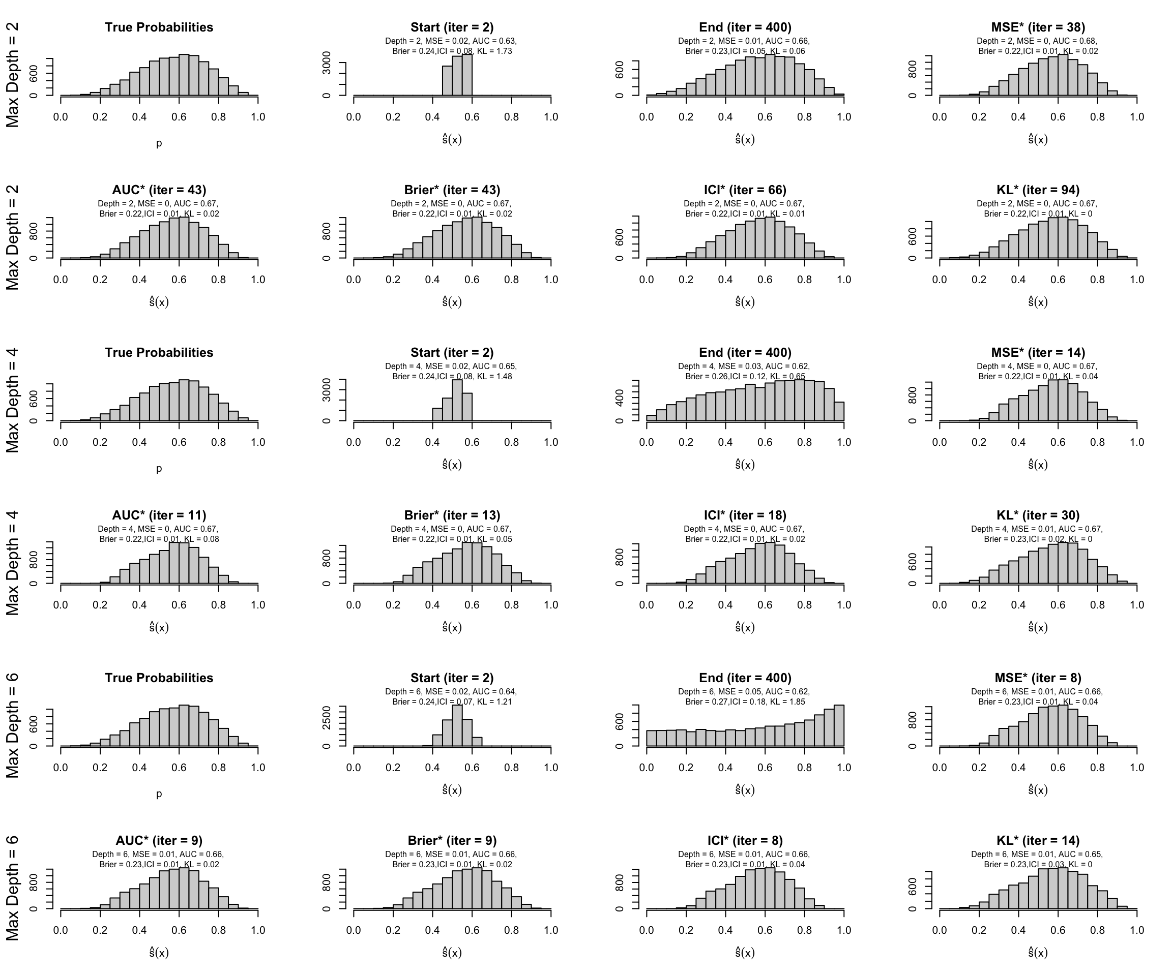
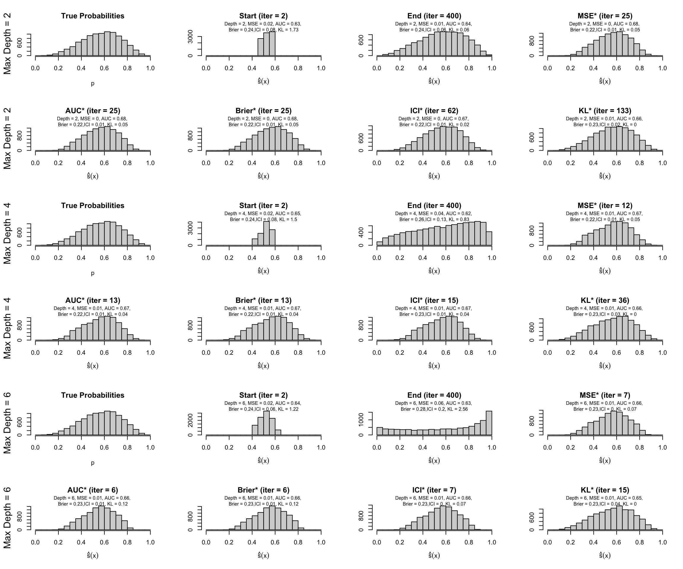
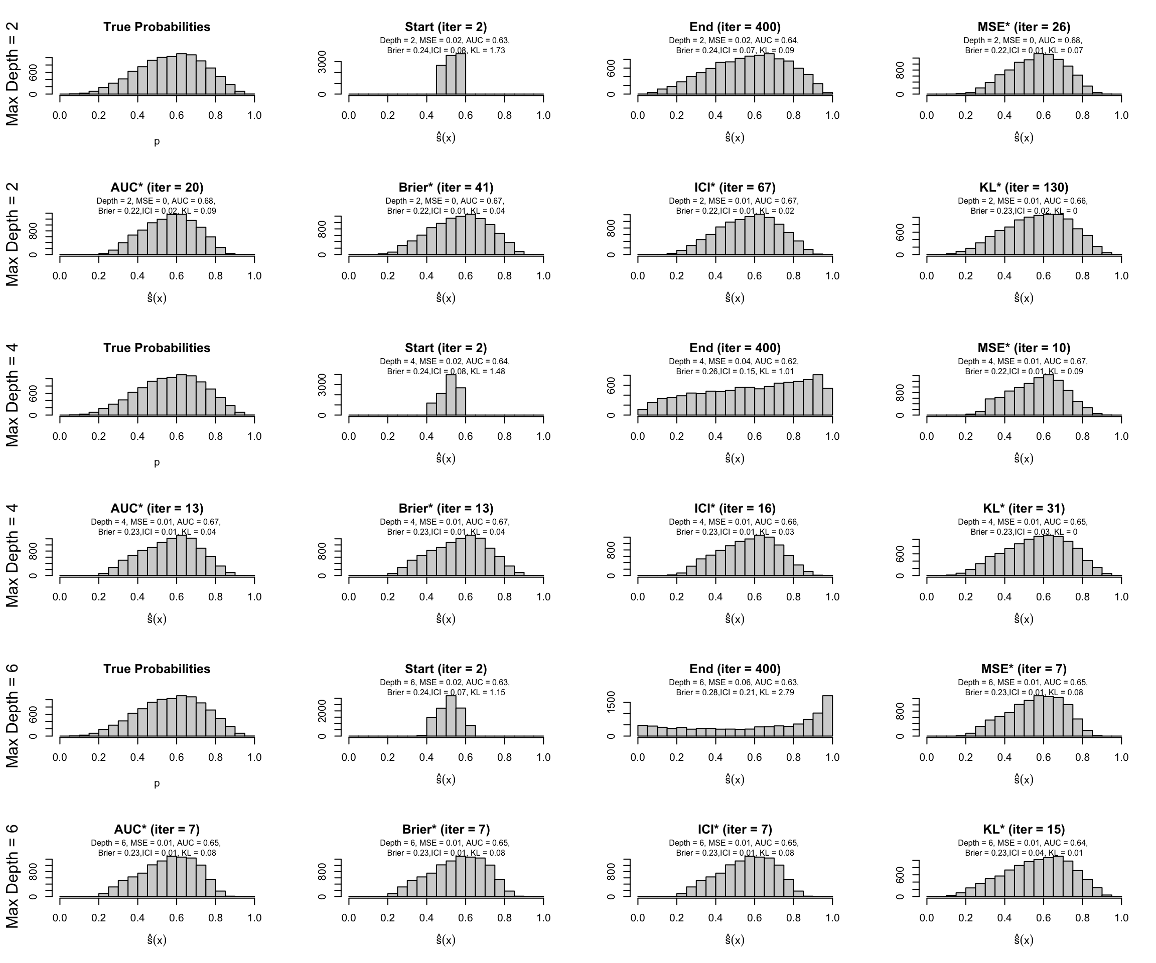
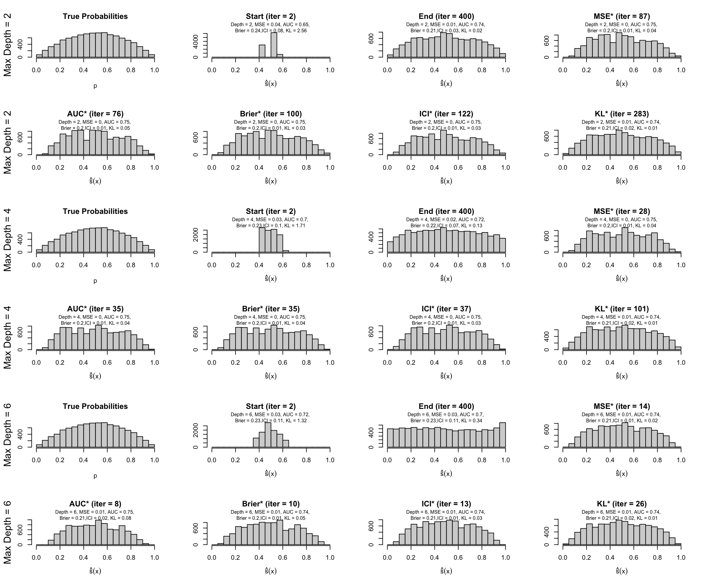
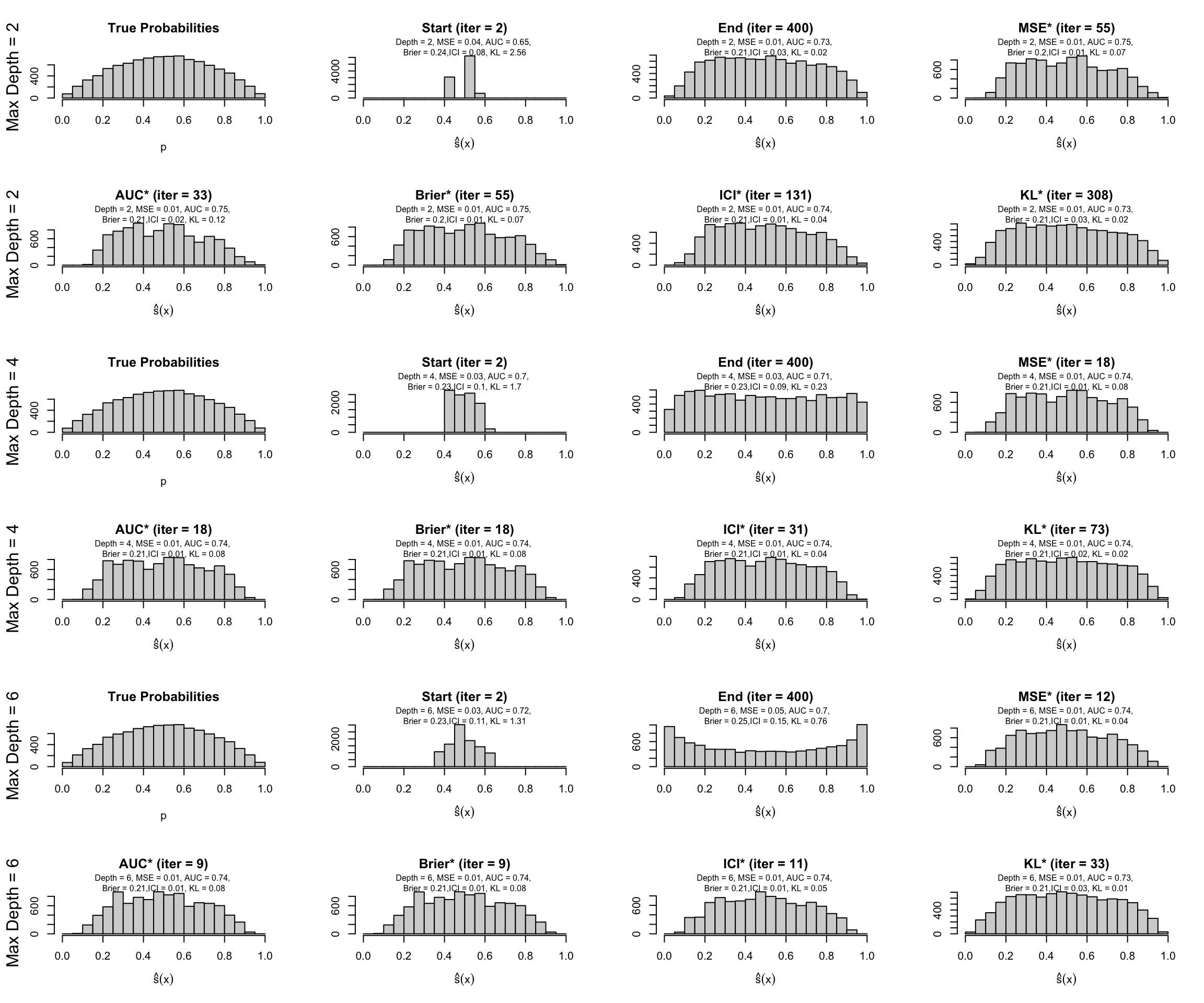
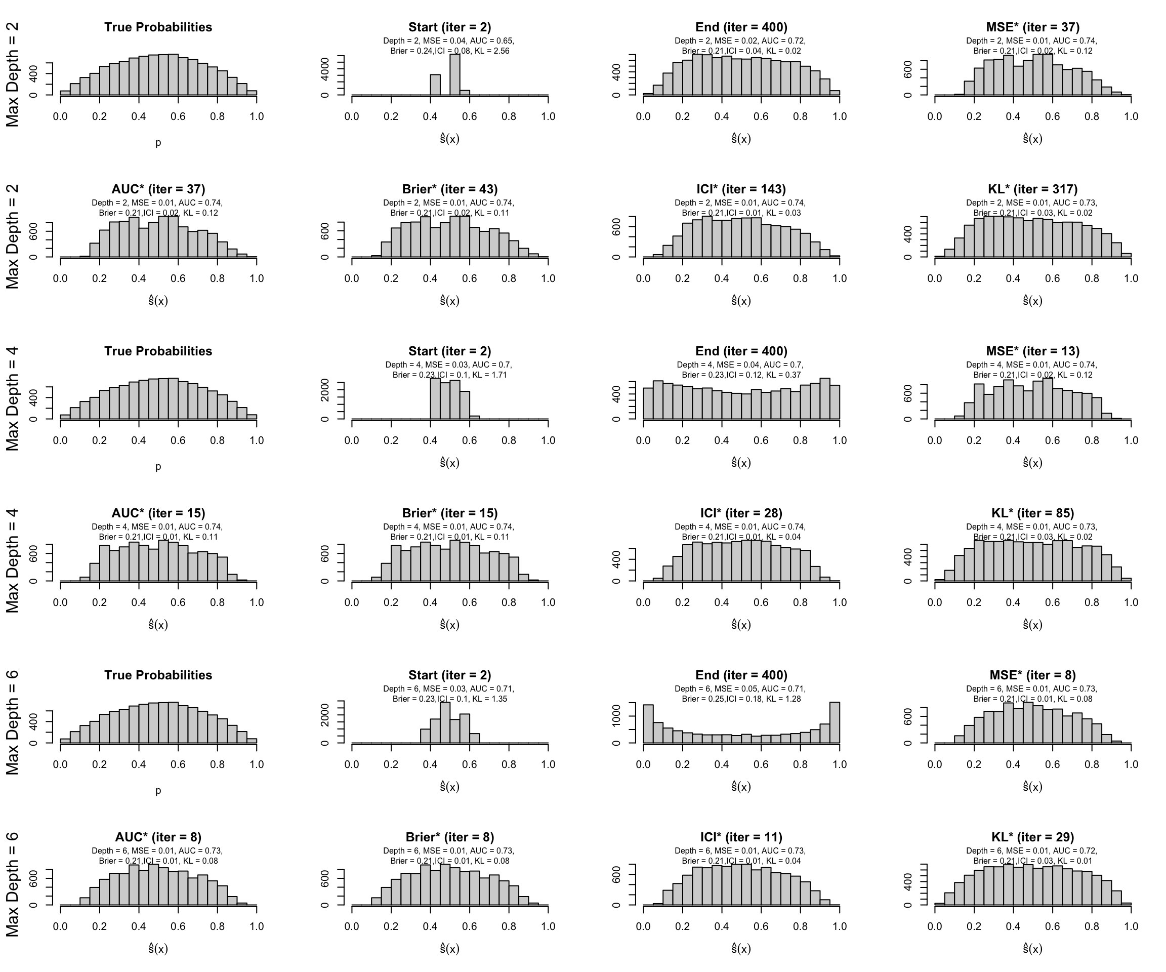
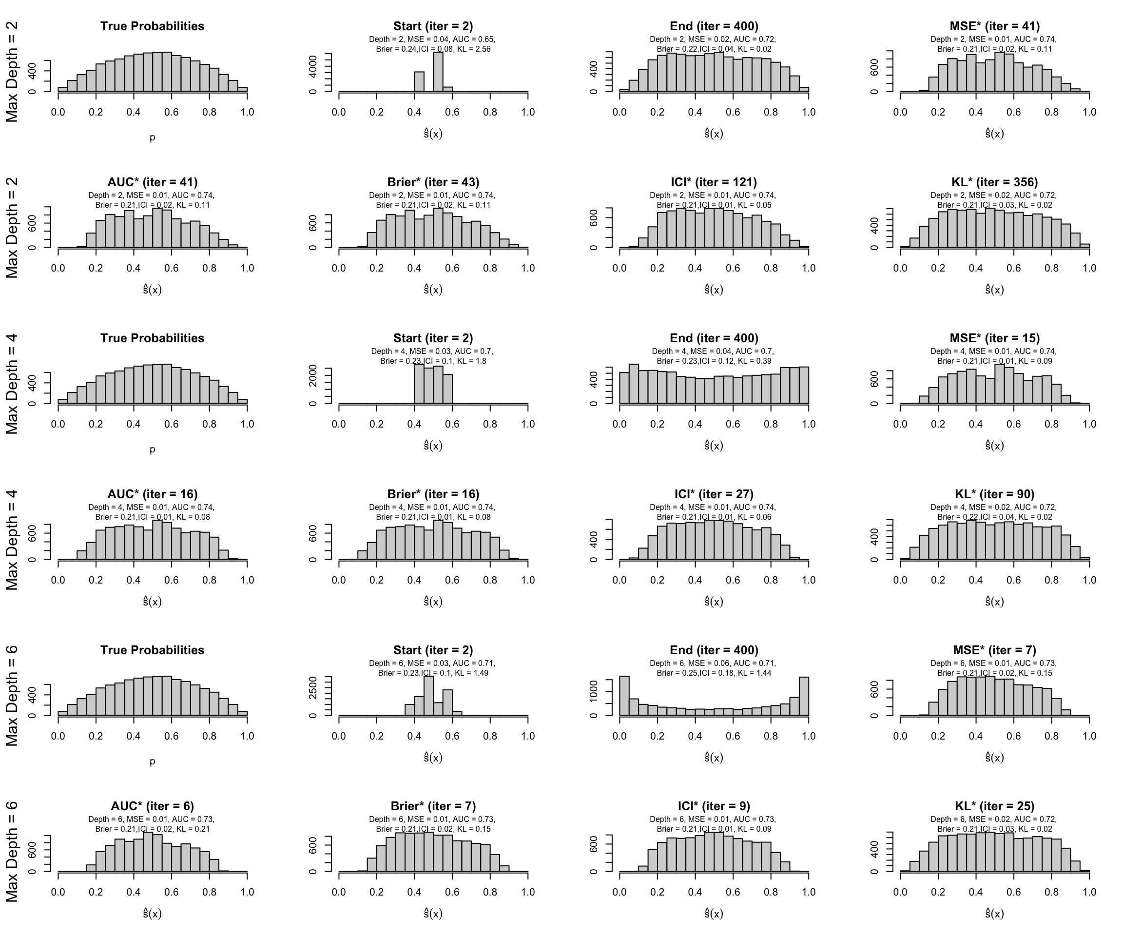
We then define a function, plot_bp_xgb() which plots the distribution of scores on the test set for a single replication (repn), for a scenario, (scenario), and a given maximal tree depth (max_depth). We also define a helper function, plot_bp_interest(), which plots the histogram of the scores at a specific iteration number. We will then be able to plot the distributions at the beginning of the boosting iterations, at the end, at a point where the AUC was the highest on the validation set, and at a point where the KL divergence between the distribution of scores on the validation set and the distribution of the true probabilities was the lowest.
Code to create the barplots
plot_bp_interest <-function(metrics_interest, scores_hist_interest, label) { subtitle <-str_c("Depth = ", metrics_interest$max_depth, ", ","MSE = ", round(metrics_interest$mse, 2), ", ","AUC = ", round(metrics_interest$AUC, 2), ", \n","Brier = ", round(metrics_interest$brier, 2), ",","ICI = ", round(metrics_interest$ici, 2), ", ","KL = ", round(metrics_interest$KL_20_true_probas, 2) )plot(main =str_c(label, " (iter = ", metrics_interest$nb_iter,")"), scores_hist_interest$test,xlab = latex2exp::TeX("$\\hat{s}(x)$"),ylab ="" )mtext(side =3, line =-0.25, adj = .5, subtitle, cex = .5)}plot_bp_xgb <-function(scenario, repn, max_depth) {# Focus on current scenario scores_hist_scenario <- scores_hist_all[[scenario]]# Focus on a particular replication scores_hist_repn <- scores_hist_scenario[[repn]]# Focus on a value for max_depth max_depth_val <-map_dbl(scores_hist_repn, ~.x[[1]]$max_depth) i_max_depth <-which(max_depth_val == max_depth) scores_hist <- scores_hist_repn[[i_max_depth]]# The metrics for the corresponding simulations, on the validation set metrics_xgb_current_valid <- metrics_xgb_all |>filter( scenario ==!!scenario, repn ==!!repn, max_depth ==!!max_depth, sample =="Validation" )# and on the test set metrics_xgb_current_test <- metrics_xgb_all |>filter( scenario ==!!scenario, repn ==!!repn, max_depth ==!!max_depth, sample =="Test" )# True Probabilities simu_data <-simulate_data_wrapper(scenario = scenario,params_df = params_df,repn = repn # only one replication here ) true_prob <- simu_data$data$probs_trainhist( true_prob,breaks =seq(0, 1, by = .05),xlab ="p", ylab ="",main ="True Probabilities",xlim =c(0, 1) )mtext(side =2, str_c("Max Depth = ", max_depth), line =2.5, cex =1,font.lab =2 )# Iterations of interest----## Start of iterations scores_hist_start <- scores_hist[[1]] metrics_start <- metrics_xgb_current_test |>filter(nb_iter == scores_hist_start$nb_iter)plot_bp_interest(metrics_interest = metrics_start,scores_hist_interest = scores_hist_start,label ="Start" )## End of iterations scores_hist_end <- scores_hist[[length(scores_hist)]] metrics_end <- metrics_xgb_current_test |>filter(nb_iter == scores_hist_end$nb_iter)plot_bp_interest(metrics_interest = metrics_end,scores_hist_interest = scores_hist_end,label ="End" )## Iteration with min MSE on validation set nb_iter_mse <- metrics_xgb_current_valid |>arrange(mse) |> dplyr::slice(1) |>pull("nb_iter")# Metrics at the same iteration on the test set metrics_min_mse <- metrics_xgb_current_test |>filter(nb_iter ==!!nb_iter_mse)# Note: indexing at 0 here... ind_mse <-which(map_dbl(scores_hist, "nb_iter") == nb_iter_mse) scores_hist_min_mse <- scores_hist[[ind_mse]]plot_bp_interest(metrics_interest = metrics_min_mse,scores_hist_interest = scores_hist_min_mse,label ="MSE*" )## Iteration with max AUC on validation set nb_iter_auc <- metrics_xgb_current_valid |>arrange(desc(AUC)) |> dplyr::slice(1) |>pull("nb_iter") metrics_max_auc <- metrics_xgb_current_test |>filter(nb_iter ==!!nb_iter_auc)# Note: indexing at 0 here... ind_auc <-which(map_dbl(scores_hist, "nb_iter") == nb_iter_auc) scores_hist_max_auc <- scores_hist[[ind_auc]]plot_bp_interest(metrics_interest = metrics_max_auc,scores_hist_interest = scores_hist_max_auc,label ="AUC*" )mtext(side =2, str_c("Max Depth = ", max_depth), line =2.5, cex =1,font.lab =2 )## Min Brier on validation set nb_iter_brier <- metrics_xgb_current_valid |>arrange(brier) |> dplyr::slice(1) |>pull("nb_iter") metrics_min_brier <- metrics_xgb_current_test |>filter(nb_iter ==!!nb_iter_brier) ind_brier <-which(map_dbl(scores_hist, "nb_iter") == nb_iter_brier) scores_hist_min_brier <- scores_hist[[ind_brier]]plot_bp_interest(metrics_interest = metrics_min_brier,scores_hist_interest = scores_hist_min_brier,label ="Brier*" )## Min ICI on validation set nb_iter_ici <- metrics_xgb_current_valid |>arrange(ici) |> dplyr::slice(1) |>pull("nb_iter") metrics_min_ici <- metrics_xgb_current_test |>filter(nb_iter ==!!nb_iter_ici) ind_ici <-which(map_dbl(scores_hist, "nb_iter") == nb_iter_ici) scores_hist_min_ici <- scores_hist[[ind_ici]]plot_bp_interest(metrics_interest = metrics_min_ici,scores_hist_interest = scores_hist_min_ici,label ="ICI*" )## Min KL on validation set nb_iter_kl <- metrics_xgb_current_valid |>arrange(KL_20_true_probas) |> dplyr::slice(1) |>pull("nb_iter") metrics_min_kl <- metrics_xgb_current_test |>filter(nb_iter ==!!nb_iter_kl) ind_kl <-which(map_dbl(scores_hist, "nb_iter") == nb_iter_kl) scores_hist_min_kl <- scores_hist[[ind_kl]]plot_bp_interest(metrics_interest = metrics_min_kl,scores_hist_interest = scores_hist_min_kl,label ="KL*" )}
Let us plot the distributions for the first replication of the simulations of each scenario.
Distribution of scores on the test set for Scenario 13.
Distribution of scores on the test set for Scenario 14.
Distribution of scores on the test set for Scenario 15.
Distribution of scores on the test set for Scenario 16.
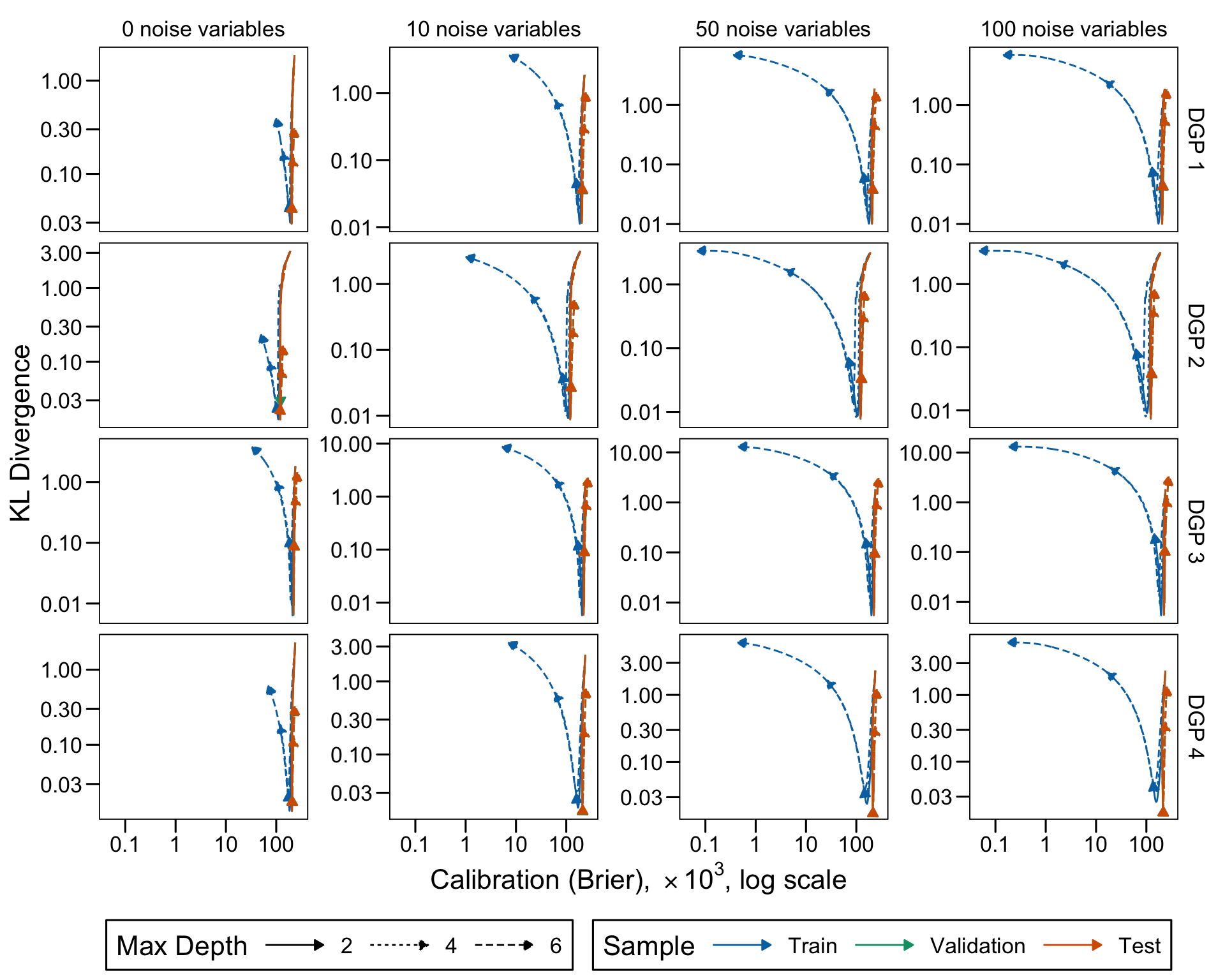
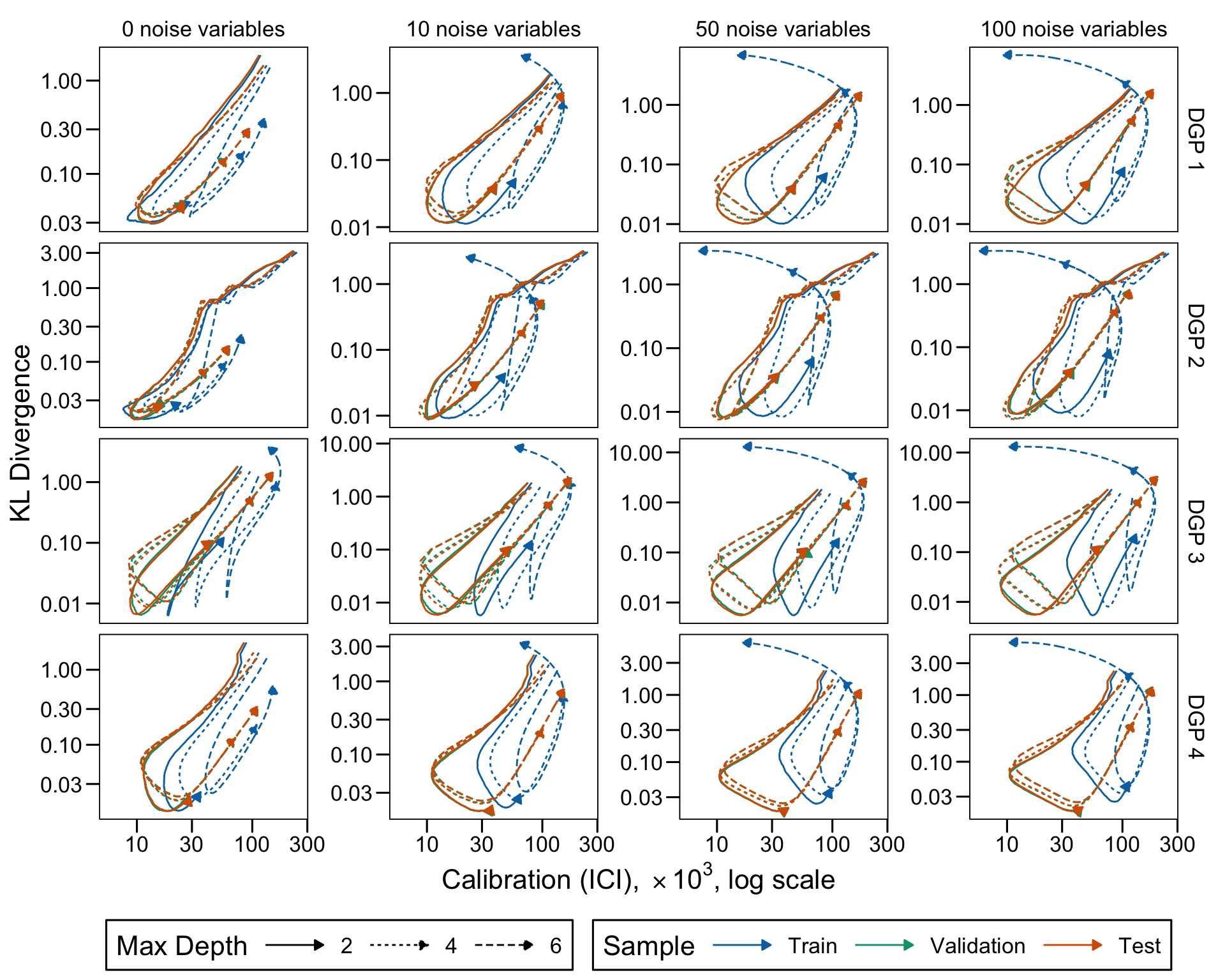
8.5.3 KL Divergence and Calibration along Boosting Iterations
We can examine the evolution of the relationship between the divergence of score distributions from true probabilities and model calibration across increasing boosting iterations.
Figure 8.6: KL Divergence and Calibration (ICI) across increasing boosting iterations (log scales)
Ojeda, Francisco M., Max L. Jansen, Alexandre Thiéry, Stefan Blankenberg, Christian Weimar, Matthias Schmid, and Andreas Ziegler. 2023. “Calibrating Machine Learning Approaches for Probability Estimation: A Comprehensive Comparison.”Statistics in Medicine 42 (29): 5451–78. https://doi.org/10.1002/sim.9921.