12  Comparison of Models

Note

This chapter loads the estimated models from the previous chapters from this simulation part of the supplementary materials and compares them.

library(tidyverse)
── Attaching core tidyverse packages ──────────────────────── tidyverse 2.0.0 ──
✔ dplyr     1.1.4     ✔ readr     2.1.5
✔ forcats   1.0.0     ✔ stringr   1.5.1
✔ ggplot2   3.5.1     ✔ tibble    3.2.1
✔ lubridate 1.9.3     ✔ tidyr     1.3.1
✔ purrr     1.0.2     
── Conflicts ────────────────────────────────────────── tidyverse_conflicts() ──
✖ dplyr::filter() masks stats::filter()
✖ dplyr::lag()    masks stats::lag()
ℹ Use the conflicted package (<http://conflicted.r-lib.org/>) to force all conflicts to become errors
library(locfit)
locfit 1.5-9.9   2024-03-01

Attaching package: 'locfit'

The following object is masked from 'package:purrr':

    none
library(philentropy)

# Colours for train/validation/test
colour_samples <- c(
  "Train" = "#0072B2",
  "Validation" = "#009E73",
  "Test" = "#D55E00"
)

# Colour for the models of interest
colour_result_type <- c(
  "AUC*" = "#D55E00", 
  "Smallest" = "#56B4E9", 
  "Largest" = "#009E73", 
  "Brier*" = "gray",
  "MSE*" = "#0072B2",
  "ICI*" = "#CC79A7", 
  "KL*" = "#E69F00",
  "None" = "black"
)
definition of the theme_paper() function (for ggplot2 graphs)
#' Theme for ggplot2
#'
#' @param ... arguments passed to the theme function
#' @export
#' @importFrom ggplot2 element_rect element_text element_blank element_line unit
#'   rel
theme_paper <- function (...) {
  ggthemes::theme_base() +
    theme(
      plot.background = element_blank(),
      legend.background = element_rect(
        fill = "transparent", linetype="solid", colour ="black"),
      legend.position = "bottom",
      legend.direction = "horizontal",
      legend.box = "horizontal",
      legend.key = element_blank()
    )
}

13 Load Previous Results

13.1 Trees

The trees estimated in Chapter 5.

files <- str_c(
  "output/simul/dgp-ojeda/resul_trees_scenario_", 1:16, ".rda"
)
resul_trees <- map(files[file.exists(files)], ~{load(.x) ; resul_trees_scenario})

We can merge the metrics tables computed for each scenario and replications for these scenarios into a single tibble.

metrics_trees_all <- map(
  resul_trees,
  function(resul_trees_sc) map(resul_trees_sc, "metrics_all") |> list_rbind()
) |>
  list_rbind() |>
  mutate(
    sample = factor(
      sample,
      levels = c("train", "valid", "test"),
      labels = c("Train", "Validation", "Test")
    )
  )

We extract the metrics from the trees of interest:

  • smallest: tree with the smallest number of leaves
  • largest: tree with the highest number of leaves
  • largest_auc: tree with the highest AUC on validation set
  • lowest_mse: tree with the lowest MSE on validation set
  • lowest_brier: tree with the lowest Brier on validation set
  • lowest_ici: tree with the lowest ICI on validation set
  • lowest_kl: tree with the lowest KL Divergence on validation set
Code to identify trees of interest
# Identify the smallest tree
smallest_tree <-
  metrics_trees_all |>
  filter(sample == "Validation") |>
  group_by(scenario, repn) |>
  arrange(nb_leaves) |>
  slice_head(n = 1) |>
  select(scenario, repn, ind, nb_leaves) |>
  mutate(result_type = "smallest") |>
  ungroup()

# Identify the largest tree
largest_tree <-
  metrics_trees_all |>
  filter(sample == "Test") |>
  group_by(scenario, repn) |> 
  arrange(desc(nb_leaves)) |>
  slice_head(n = 1) |>
  select(scenario, repn, ind, nb_leaves) |>
  mutate(result_type = "largest") |> 
  ungroup()

# Identify tree with highest AUC on test set
highest_auc_tree <-
  metrics_trees_all |>
  filter(sample == "Validation") |>
  group_by(scenario, repn) |>
  arrange(desc(AUC)) |>
  slice_head(n = 1) |>
  select(scenario, repn, ind, nb_leaves) |>
  mutate(result_type = "largest_auc") |>
  ungroup()

# Identify tree with lowest MSE
lowest_mse_tree <-
  metrics_trees_all |>
  filter(sample == "Validation") |>
  group_by(scenario, repn) |>
  arrange(mse) |>
  slice_head(n = 1) |>
  select(scenario, repn, ind, nb_leaves) |>
  mutate(result_type = "lowest_mse") |>
  ungroup()

# Identify tree with lowest ICI
lowest_ici_tree <-
  metrics_trees_all |>
  filter(sample == "Validation") |>
  group_by(scenario, repn) |>
  arrange(ici) |>
  slice_head(n = 1) |>
  select(scenario, repn, ind, nb_leaves) |>
  mutate(result_type = "lowest_ici") |>
  ungroup()

# Identify tree with lowest Brier's score
lowest_brier_tree <-
  metrics_trees_all |>
  filter(sample == "Validation") |>
  group_by(scenario, repn) |>
  arrange(brier) |>
  slice_head(n = 1) |>
  select(scenario, repn, ind, nb_leaves) |>
  mutate(result_type = "lowest_brier") |>
  ungroup()

# Identify tree with lowest KL
lowest_kl_tree <-
  metrics_trees_all |>
  filter(sample == "Validation") |>
  group_by(scenario, repn) |>
  arrange(KL_20_true_probas) |>
  slice_head(n = 1) |>
  select(scenario, repn, ind, nb_leaves) |>
  mutate(result_type = "lowest_kl") |>
  ungroup()


# Merge these
trees_of_interest_tree <-
  smallest_tree |>
  bind_rows(largest_tree) |>
  bind_rows(highest_auc_tree) |>
  bind_rows(lowest_mse_tree) |>
  bind_rows(lowest_ici_tree) |>
  bind_rows(lowest_brier_tree) |>
  bind_rows(lowest_kl_tree)

# Add metrics now
trees_of_interest_metrics_tree <-
  trees_of_interest_tree |>
  left_join(
    metrics_trees_all, 
    by = c("scenario", "repn", "ind", "nb_leaves"),
    relationship = "many-to-many" # (train, valid, test)
  ) |> 
  mutate(
    result_type = factor(
      result_type,
      levels = c(
        "smallest", "largest", "lowest_mse", "largest_auc",
        "lowest_brier", "lowest_ici", "lowest_kl"),
      labels = c(
        "Smallest", "Largest", "MSE*", "AUC*", 
        "Brier*", "ICI*", "KL*"
      )
    )
  )

# Sanity check
# trees_of_interest_metrics_tree |> count(scenario, sample, result_type)

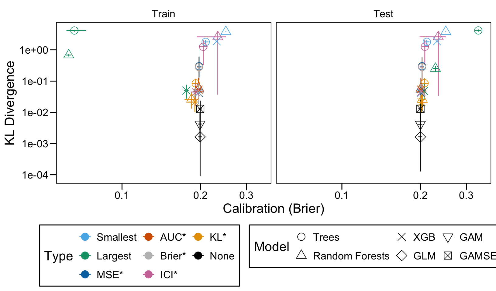
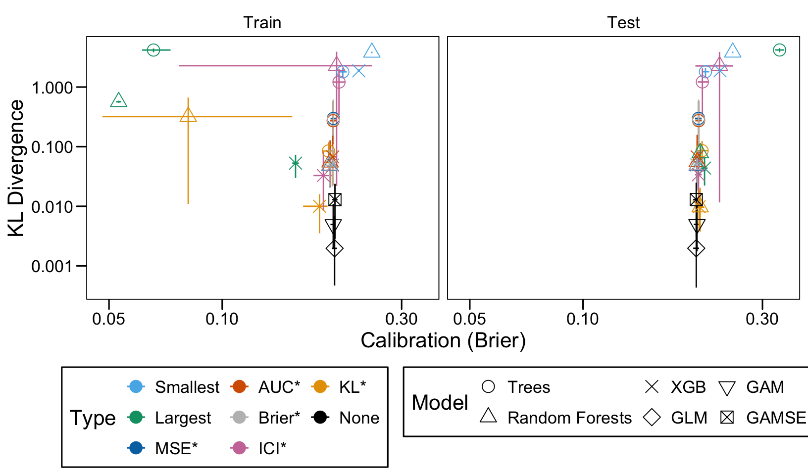
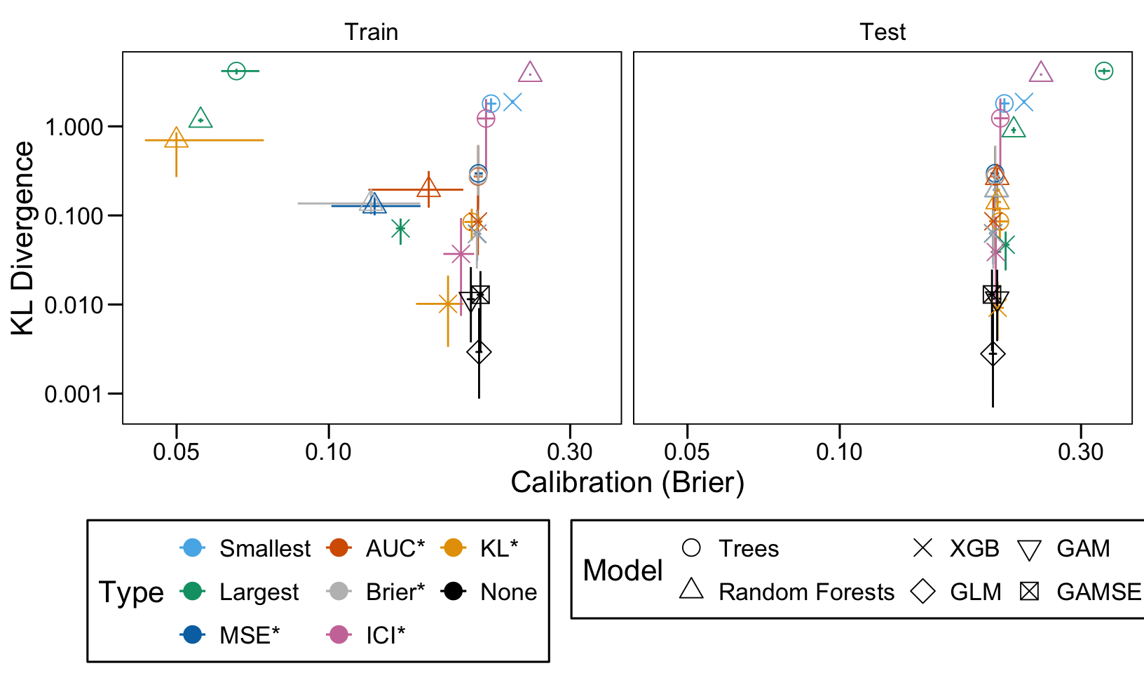
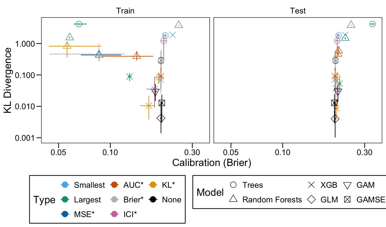
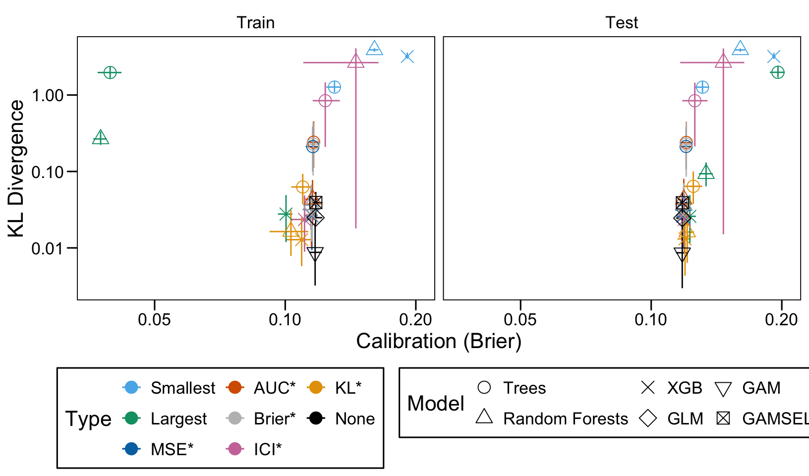
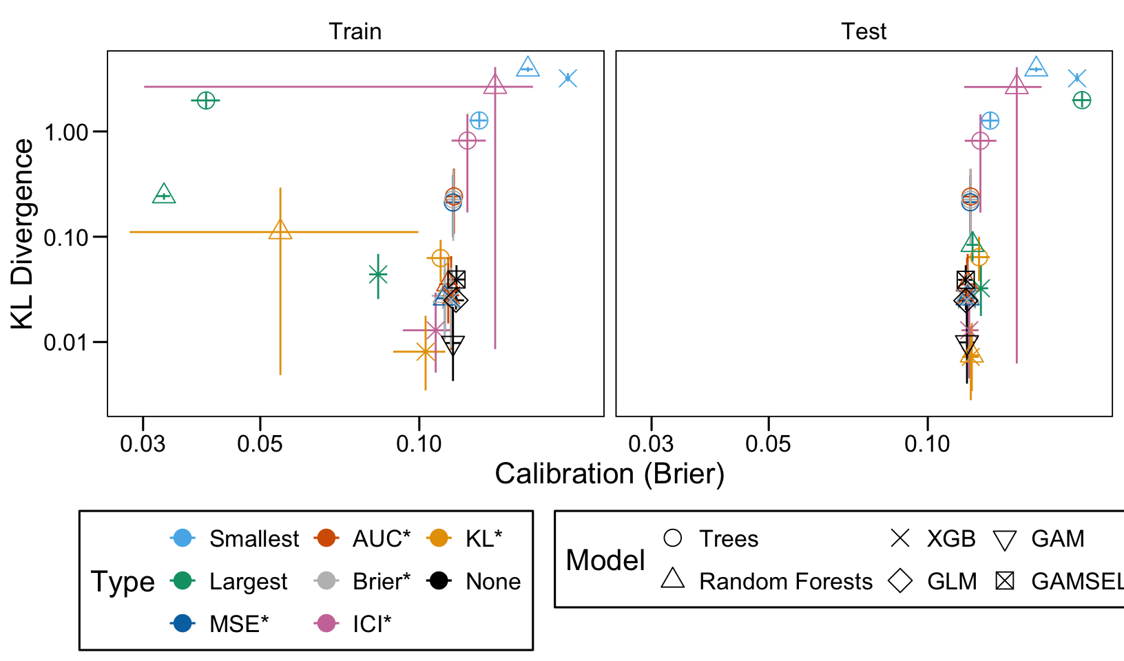
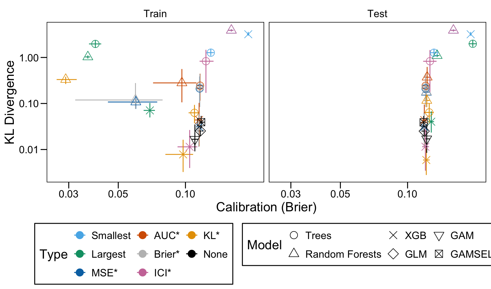
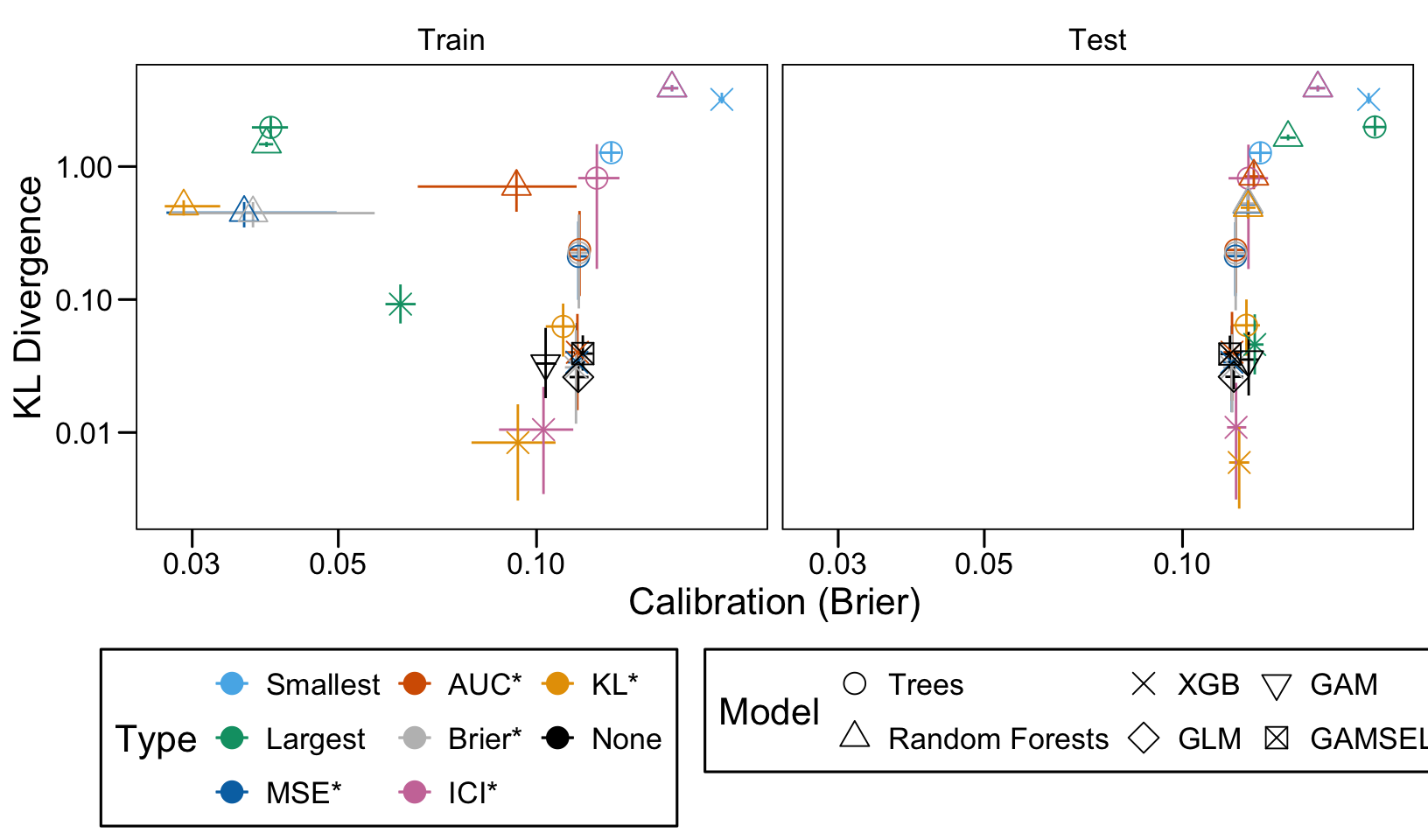
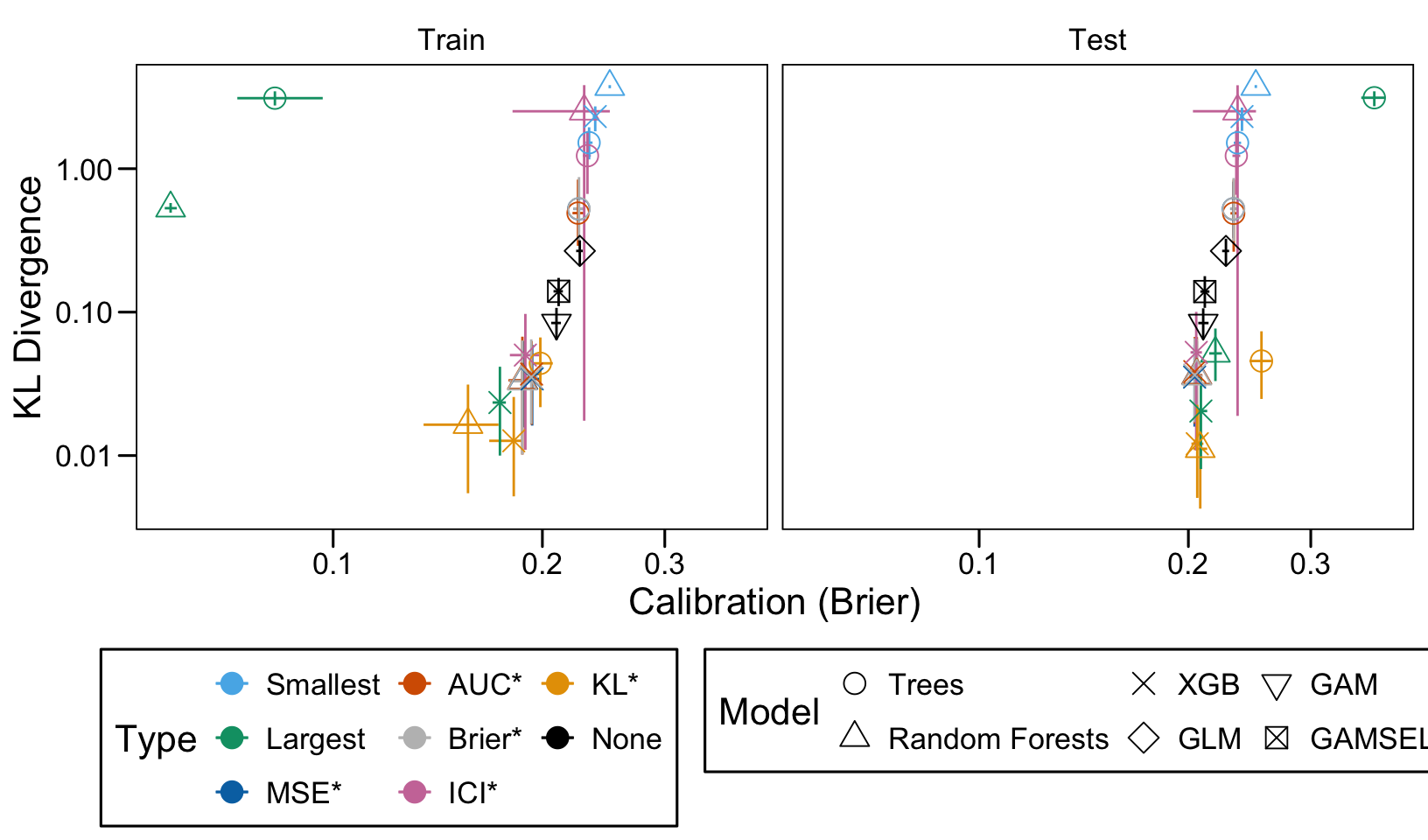
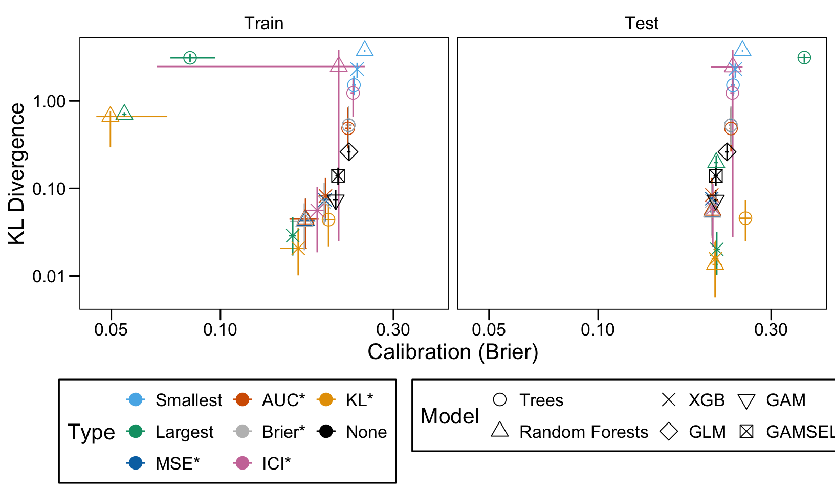
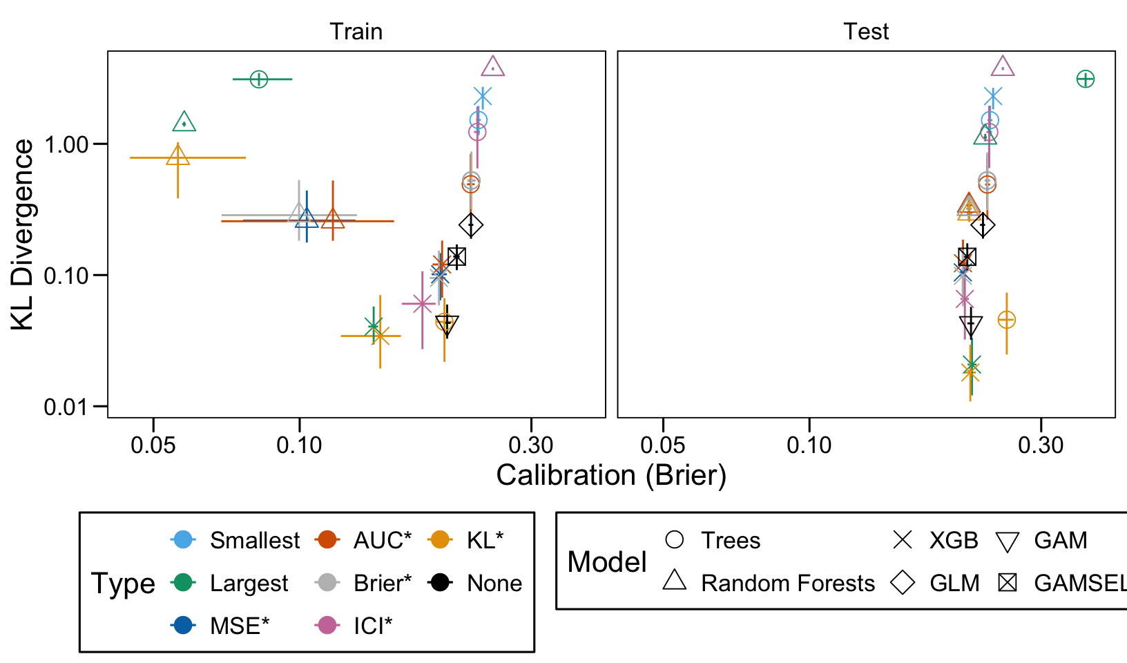
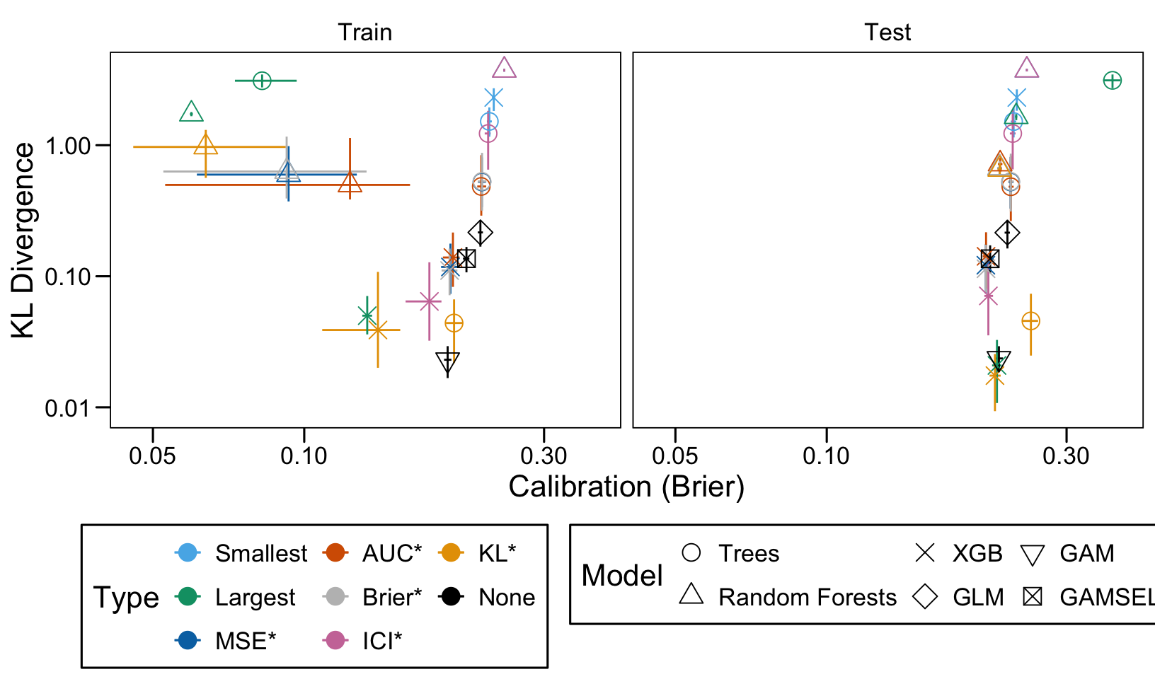
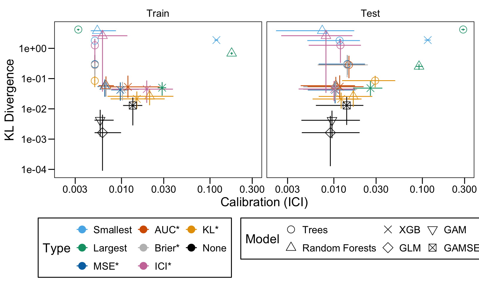
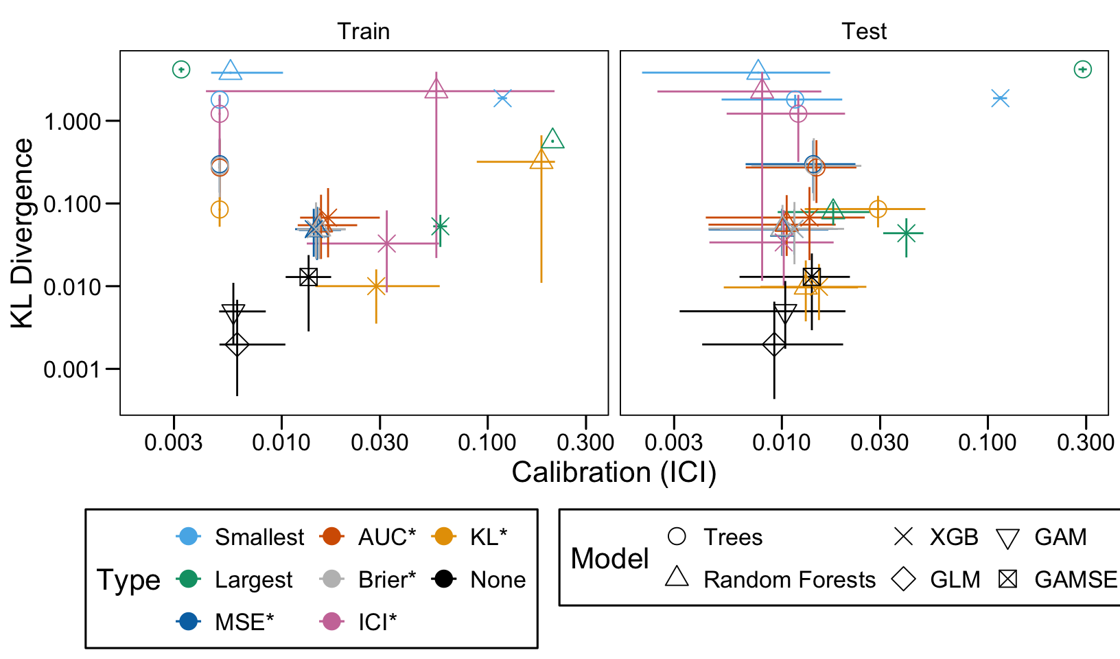
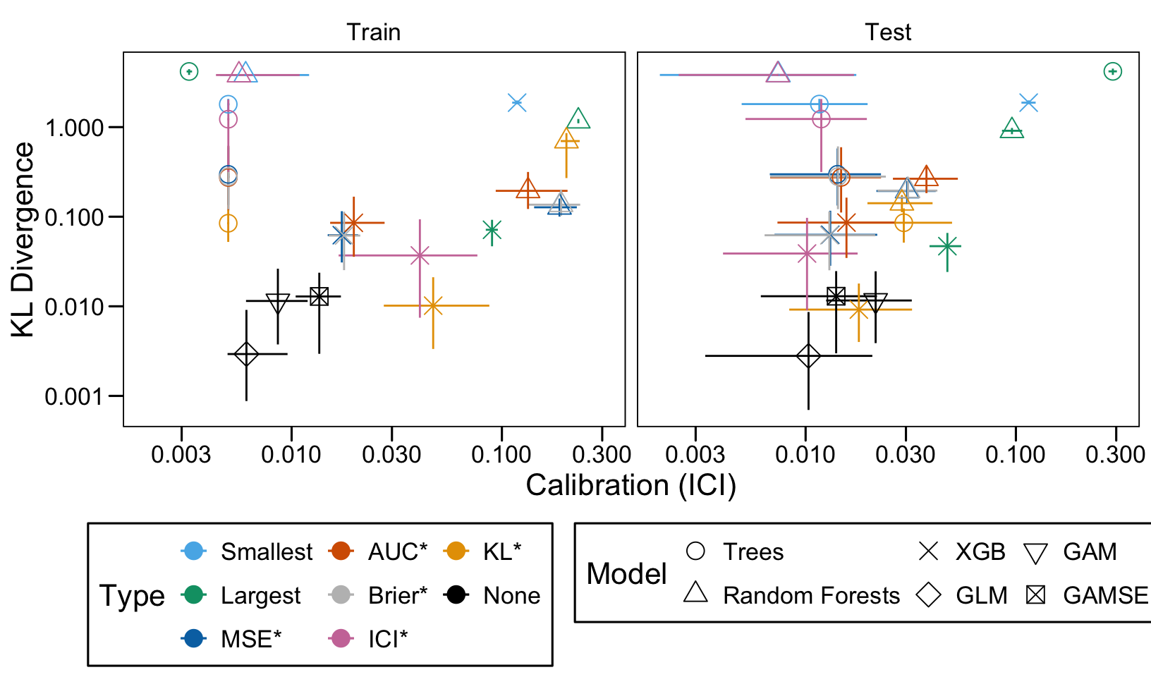
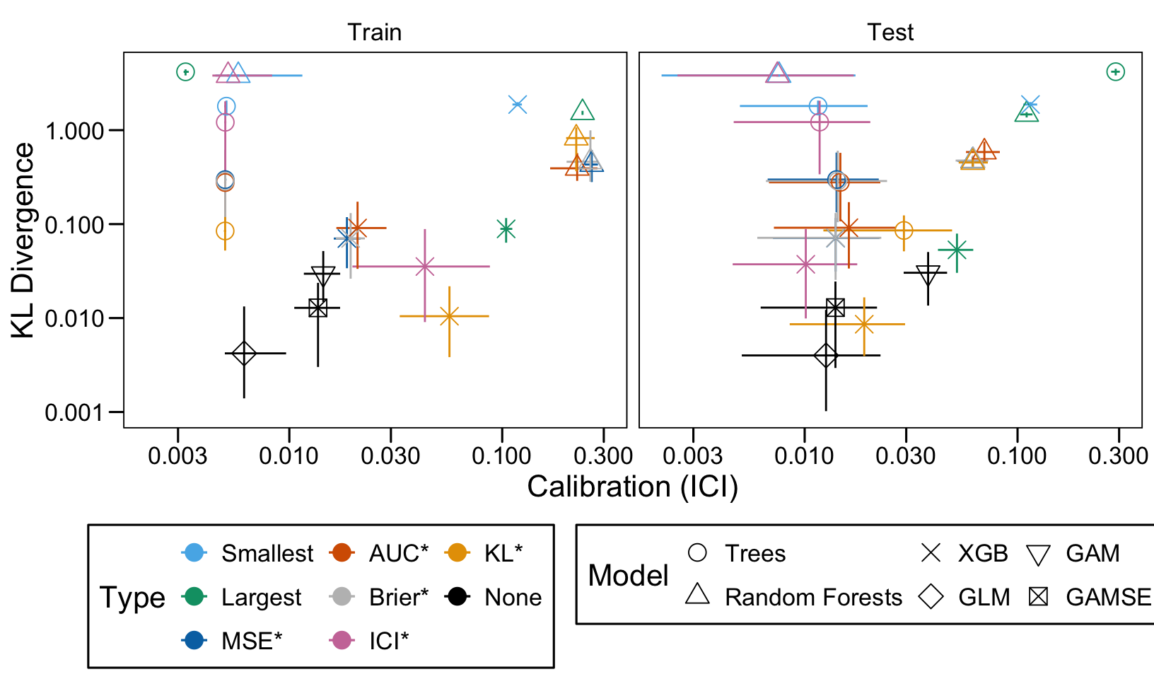
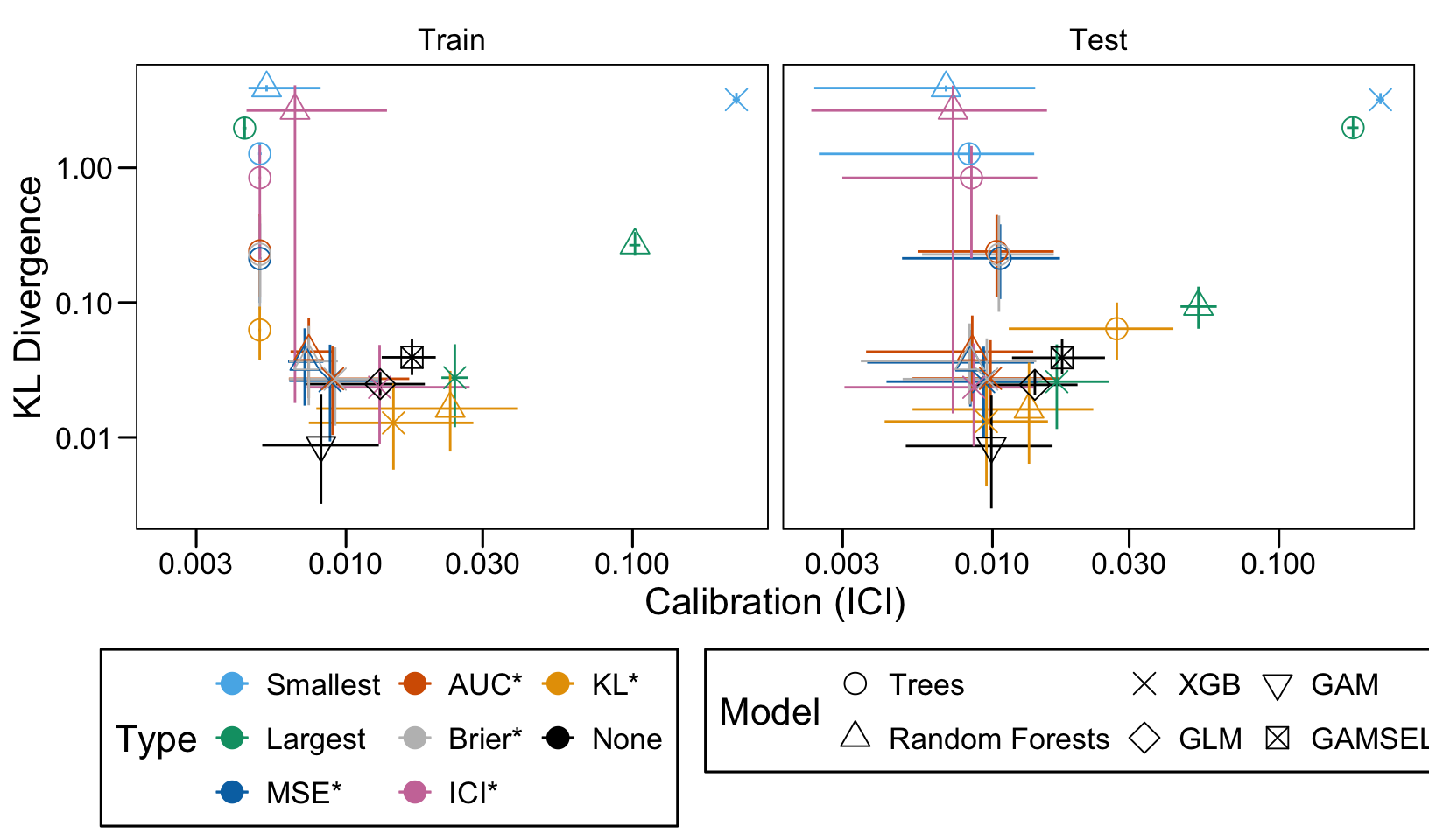
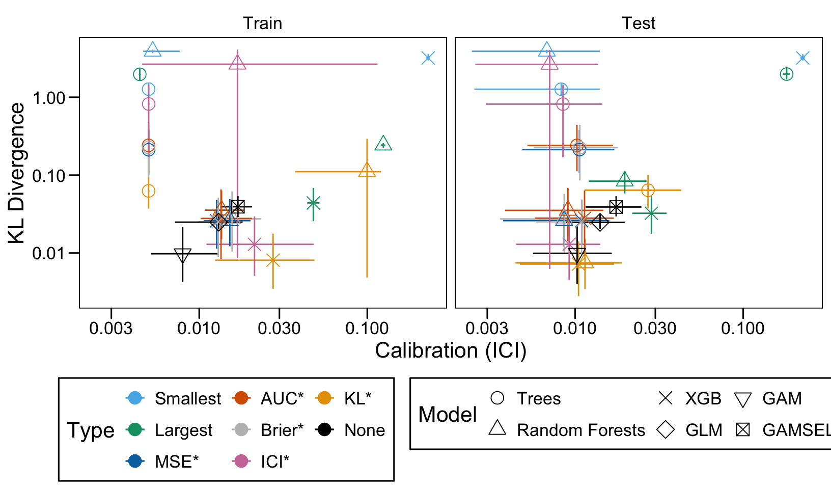
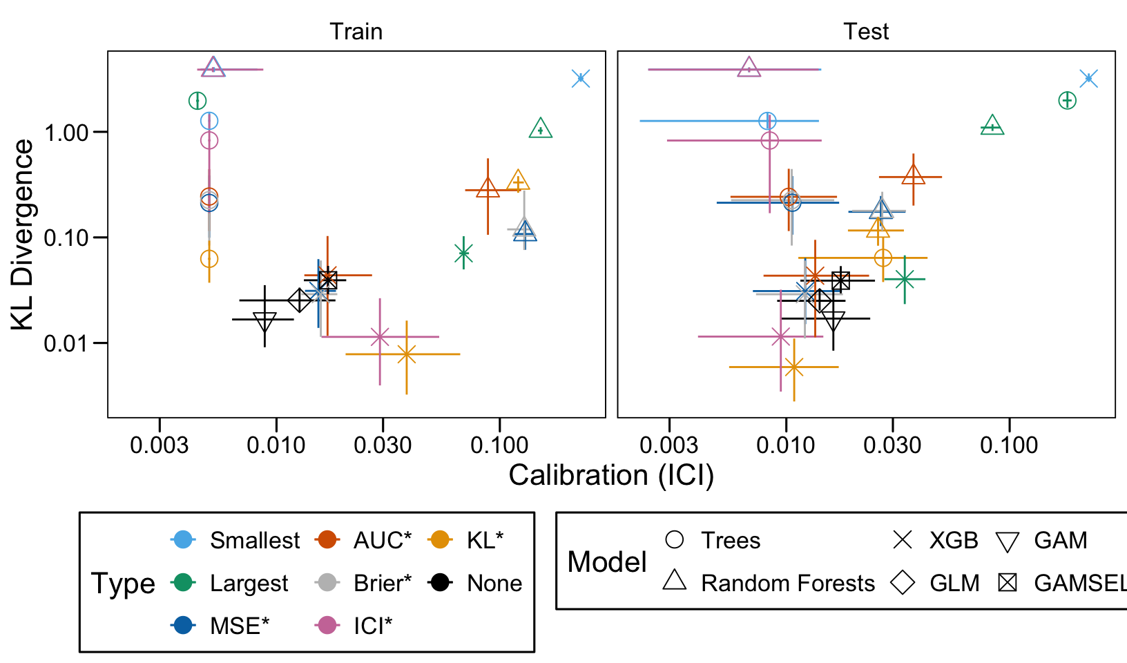
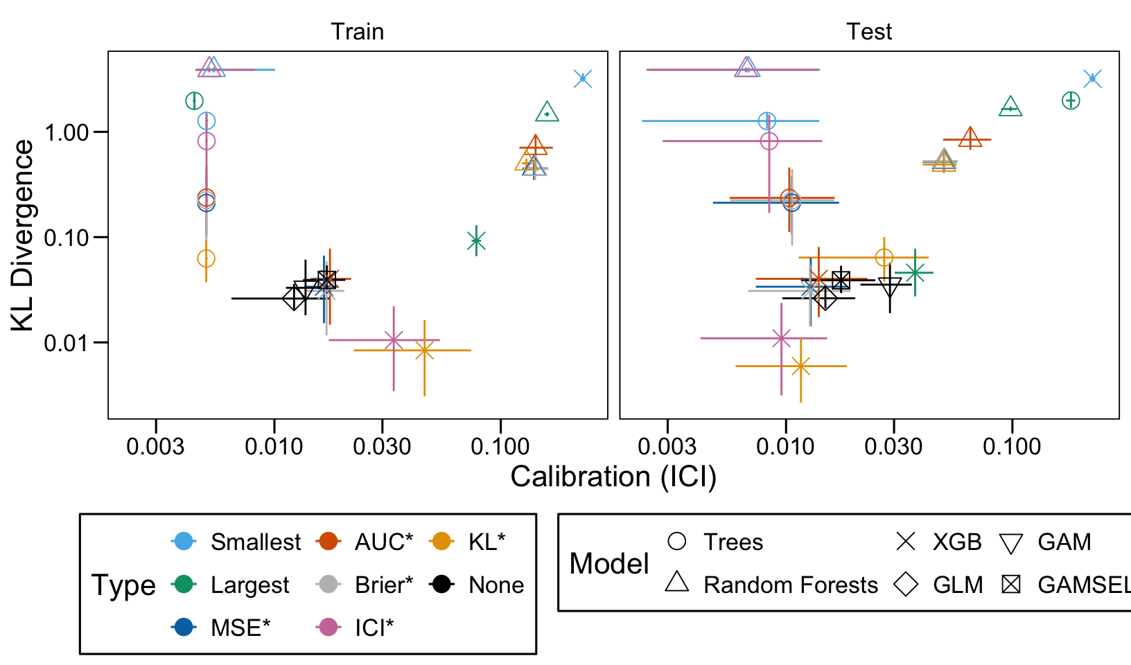
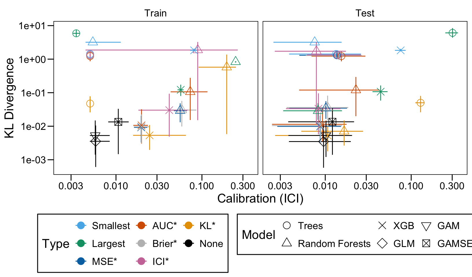
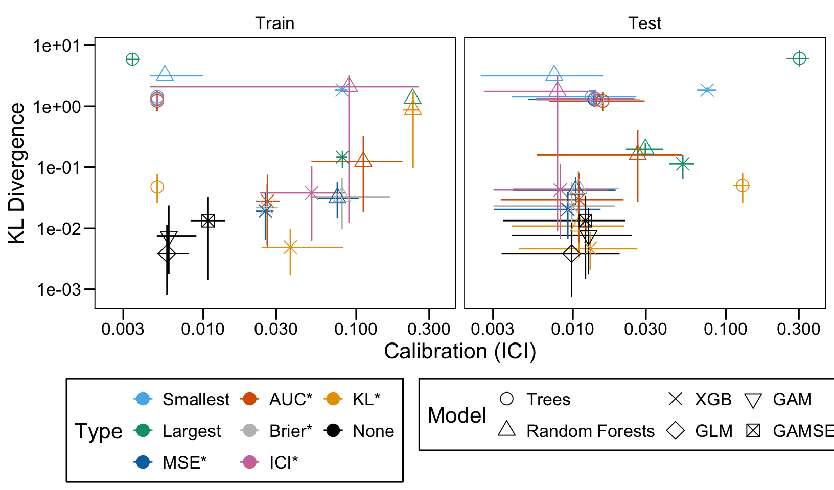
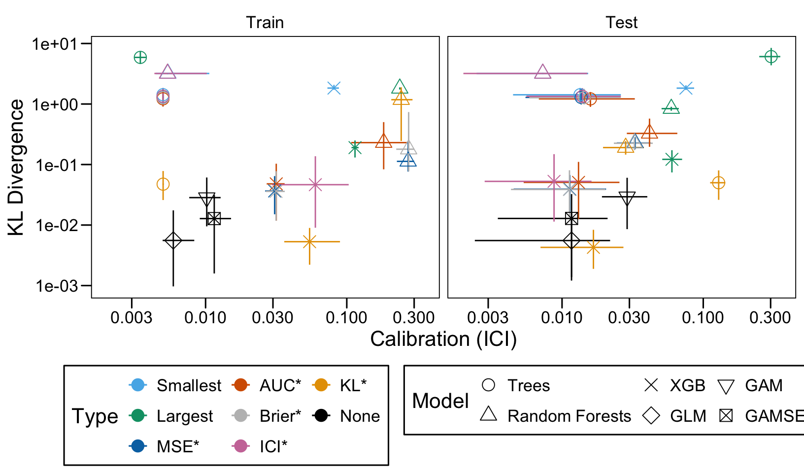
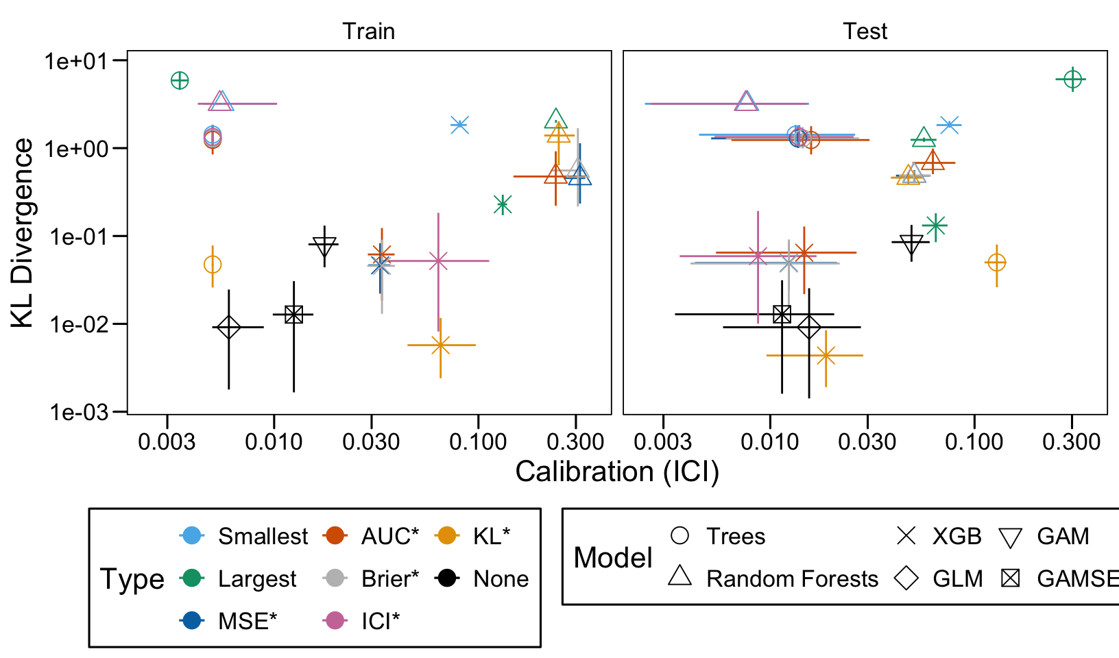
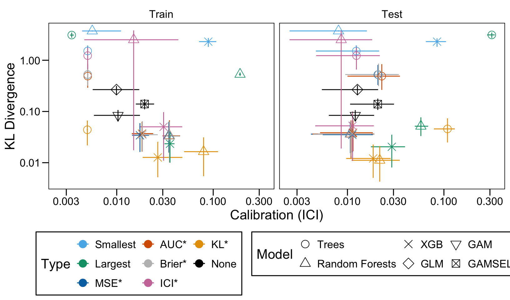
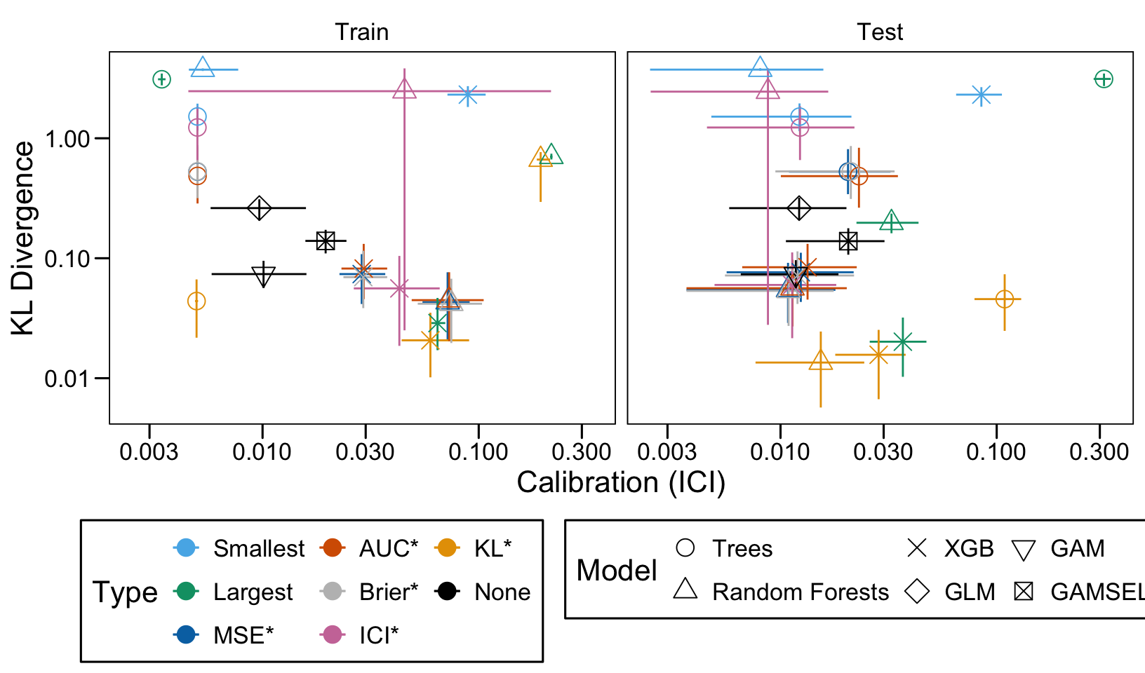
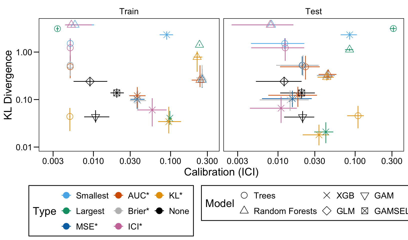
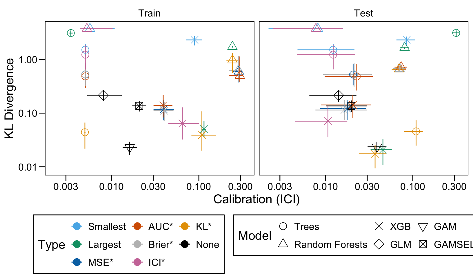
We ran 100 replications of the simulations for each scenario. Let us compute the average AUC, ICI and KL Divergence over these 100 replications, both on the train and on the validation set.

models_interest_trees <- 
  trees_of_interest_metrics_tree |> 
  group_by(scenario, sample, result_type) |> 
  summarise(
    AUC_lower = quantile(AUC, probs = 2.5/100),
    AUC_upper = quantile(AUC, probs = 97.5/100),
    AUC_sd = sd(AUC),
    AUC = mean(AUC),
    brier_lower = quantile(brier, probs = 2.5/100),
    brier_upper = quantile(brier, probs = 97.5/100),
    brier_sd = sd(brier),
    brier = mean(brier),
    ici_lower = quantile(ici, probs = 2.5/100),
    ici_upper = quantile(ici, probs = 97.5/100),
    ici_sd = sd(ici),
    ici = mean(ici),
    KL_20_true_probas_lower = quantile(KL_20_true_probas, probs = 2.5/100),
    KL_20_true_probas_upper = quantile(KL_20_true_probas, probs = 97.5/100),
    KL_20_true_probas_sd = sd(KL_20_true_probas),
    KL_20_true_probas = mean(KL_20_true_probas),
    quant_ratio_sd = sd(inter_quantile_10_90),
    quant_ratio = mean(inter_quantile_10_90),
    .groups = "drop"
  ) |> 
  mutate(model = "tree")

13.2 Random Forests

We load the estimated random forests from Chapter 6.

files <- str_c(
  "output/simul/dgp-ojeda/resul_rf_scenario_", 1:16, ".rda"
)
resul_rf <- map(files[file.exists(files)], ~{load(.x) ; resul_rf_scenario})

Let us merge in a single tibble the metrics computed over the replications of the scenarios.

metrics_rf_all <- map(
  resul_rf,
  function(resul_rf_sc) map(resul_rf_sc, "metrics_all") |> list_rbind()
) |>
  list_rbind() |>
  mutate(
    sample = factor(
      sample,
      levels = c("train", "test", "valid"),
      labels = c("Train", "Test", "Validation")
    )
  )

We extract the metrics from the trees of interest:

  • smallest: forest with the smallest average number of leaves in the trees
  • largest: forest with the highest average number of leaves in the trees
  • largest_auc: forest with the highest AUC on validation set
  • lowest_mse: forest with the lowest MSE on validation set
  • lowest_ici: forest with the lowest ICI on validation set
  • lowest_brier: forest with the lowest Brier score on validation set
  • lowest_kl: forest with the lowest KL Divergence on validation set
Code
# Identify the model with the smallest number of leaves on average on
# validation set
smallest_rf <-
  metrics_rf_all |>
  filter(sample == "Validation") |>
  group_by(scenario, repn) |>
  arrange(nb_leaves) |>
  slice_head(n = 1) |>
  select(scenario, repn, ind, nb_leaves) |>
  mutate(result_type = "smallest") |>
  ungroup()

# Identify the largest tree
largest_rf <-
  metrics_rf_all |>
  filter(sample == "Validation") |>
  group_by(scenario, repn) |>
  arrange(desc(nb_leaves)) |>
  slice_head(n = 1) |>
  select(scenario, repn, ind, nb_leaves) |>
  mutate(result_type = "largest") |>
  ungroup()

# Identify tree with highest AUC on test set
highest_auc_rf <-
  metrics_rf_all |>
  filter(sample == "Validation") |>
  group_by(scenario, repn) |>
  arrange(desc(AUC)) |>
  slice_head(n = 1) |>
  select(scenario, repn, ind, nb_leaves) |>
  mutate(result_type = "largest_auc") |>
  ungroup()

# Identify tree with lowest MSE
lowest_mse_rf <-
  metrics_rf_all |>
  filter(sample == "Validation") |>
  group_by(scenario, repn) |>
  arrange(mse) |>
  slice_head(n = 1) |>
  select(scenario, repn, ind, nb_leaves) |>
  mutate(result_type = "lowest_mse") |>
  ungroup()

# Identify tree with lowest Brier
lowest_brier_rf <-
  metrics_rf_all |>
  filter(sample == "Validation") |>
  group_by(scenario, repn) |>
  arrange(brier) |>
  slice_head(n = 1) |>
  select(scenario, repn, ind, nb_leaves) |>
  mutate(result_type = "lowest_brier") |>
  ungroup()

# Identify tree with lowest ICI
lowest_ici_rf <-
  metrics_rf_all |>
  filter(sample == "Validation") |>
  group_by(scenario, repn) |>
  arrange(ici) |>
  slice_head(n = 1) |>
  select(scenario, repn, ind, nb_leaves) |>
  mutate(result_type = "lowest_ici") |>
  ungroup()

# Identify tree with lowest KL
lowest_kl_rf <-
  metrics_rf_all |>
  filter(sample == "Validation") |>
  group_by(scenario, repn) |>
  arrange(KL_20_true_probas) |>
  slice_head(n = 1) |>
  select(scenario, repn, ind, nb_leaves) |>
  mutate(result_type = "lowest_kl") |>
  ungroup()

# Merge these
rf_of_interest <-
  smallest_rf |>
  bind_rows(largest_rf) |>
  bind_rows(highest_auc_rf) |>
  bind_rows(lowest_mse_rf) |>
  bind_rows(lowest_brier_rf) |>
  bind_rows(lowest_ici_rf) |>
  bind_rows(lowest_kl_rf)

# Add metrics now
rf_of_interest <-
  rf_of_interest |>
  left_join(
    metrics_rf_all,
    by = c("scenario", "repn", "ind", "nb_leaves"),
    relationship = "many-to-many" # (train, valid, test)
  ) |>
  mutate(
    result_type = factor(
      result_type,
      levels = c(
        "smallest", "largest", "lowest_mse", "largest_auc",
        "lowest_brier", "lowest_ici", "lowest_kl"),
      labels = c(
        "Smallest", "Largest", "MSE*", "AUC*",
        "Brier*", "ICI*", "KL*"
      )
    )
  )

# Sanity check
# trees_of_interest_metrics_rf |> count(scenario, sample, result_type)

We ran 100 replications of the simulations for each scenario and each set of hyperparameters. Let us compute the average AUC, ICI and KL Divergence over these replications, both on the train and on the validation set.

models_interest_rf <- rf_of_interest |> 
  group_by(scenario, sample, result_type) |> 
  summarise(
    AUC_lower = quantile(AUC, probs = 2.5/100),
    AUC_upper = quantile(AUC, probs = 97.5/100),
    AUC_sd = sd(AUC),
    AUC = mean(AUC),
    brier_lower = quantile(brier, probs = 2.5/100),
    brier_upper = quantile(brier, probs = 97.5/100),
    brier_sd = sd(brier),
    brier = mean(brier),
    ici_lower = quantile(ici, probs = 2.5/100),
    ici_upper = quantile(ici, probs = 97.5/100),
    ici_sd = sd(ici),
    ici = mean(ici),
    KL_20_true_probas_lower = quantile(KL_20_true_probas, probs = 2.5/100),
    KL_20_true_probas_upper = quantile(KL_20_true_probas, probs = 97.5/100),
    KL_20_true_probas_sd = sd(KL_20_true_probas),
    KL_20_true_probas = mean(KL_20_true_probas),
    quant_ratio_sd = sd(inter_quantile_10_90),
    quant_ratio = mean(inter_quantile_10_90),
    .groups = "drop"
  ) |> 
  mutate(model = "rf")

13.3 Extreme Gradient Boosting

scenarios <- 1:16

Let us load the estimated models from Chapter 8.

files <- str_c(
  "output/simul/dgp-ojeda/resul_xgb_scenario_", scenarios, ".rda"
)
resul_xgb <- map(files[file.exists(files)], ~{load(.x) ; resul_xgb_scenario})

Let us merge in a single tibble the metrics computed over the replications of the scenarios.

metrics_xgb_all <- map(
  resul_xgb,
  function(resul_xgb_sc) map(resul_xgb_sc, "metrics_simul") |> list_rbind()
) |>
  list_rbind() |>
  mutate(
    sample = factor(
      sample,
      levels = c("train", "valid", "test"),
      labels = c("Train","Validation" ,"Test")
    )
  )

For each replication, we made some hyperparameters vary. Let us identify some models of interest:

  • smallest: model with the lowest number of boosting iteration
  • largest: model with the highest number of boosting iteration
  • largest_auc: model with the highest AUC on validation set
  • lowest_mse: model with the lowest MSE on validation set
  • lowest_brier: model with the lowest Brier score on validation set
  • lowest_ici: model with the lowest ICI on validation set
  • lowest_kl: model with the lowest KL Divergence on validation set
Code
# Identify the model with the smallest number of boosting iterations
smallest_xgb <-
  metrics_xgb_all |>
  filter(sample == "Validation") |>
  group_by(scenario, repn) |>
  arrange(nb_iter) |>
  slice_head(n = 1) |>
  select(scenario, repn, ind, nb_iter) |>
  mutate(result_type = "smallest") |>
  ungroup()

# Identify the largest tree
largest_xgb <-
  metrics_xgb_all |>
  filter(sample == "Validation") |>
  group_by(scenario, repn) |>
  arrange(desc(nb_iter)) |>
  slice_head(n = 1) |>
  select(scenario, repn, ind, nb_iter) |>
  mutate(result_type = "largest") |>
  ungroup()

# Identify tree with highest AUC on test set
highest_auc_xgb <-
  metrics_xgb_all |>
  filter(sample == "Validation") |>
  group_by(scenario, repn) |>
  arrange(desc(AUC)) |>
  slice_head(n = 1) |>
  select(scenario, repn, ind, nb_iter) |>
  mutate(result_type = "largest_auc") |>
  ungroup()

# Identify tree with lowest MSE
lowest_mse_xgb <-
  metrics_xgb_all |>
  filter(sample == "Validation") |>
  group_by(scenario, repn) |>
  arrange(mse) |>
  slice_head(n = 1) |>
  select(scenario, repn, ind, nb_iter) |>
  mutate(result_type = "lowest_mse") |>
  ungroup()

# Identify tree with lowest brier
lowest_brier_xgb <-
  metrics_xgb_all |>
  filter(sample == "Validation") |>
  group_by(scenario, repn) |>
  arrange(brier) |>
  slice_head(n = 1) |>
  select(scenario, repn, ind, nb_iter) |>
  mutate(result_type = "lowest_brier") |>
  ungroup()

# Identify tree with lowest ICI
lowest_ici_xgb <-
  metrics_xgb_all |>
  filter(sample == "Validation") |>
  group_by(scenario, repn) |>
  arrange(ici) |>
  slice_head(n = 1) |>
  select(scenario, repn, ind, nb_iter) |>
  mutate(result_type = "lowest_ici") |>
  ungroup()

# Identify tree with lowest KL
lowest_kl_xgb <-
  metrics_xgb_all |>
  filter(sample == "Validation") |>
  group_by(scenario, repn) |>
  arrange(KL_20_true_probas) |>
  slice_head(n = 1) |>
  select(scenario, repn, ind, nb_iter) |>
  mutate(result_type = "lowest_kl") |>
  ungroup()

# Merge these
models_of_interest_xgb <-
  smallest_xgb |>
  bind_rows(largest_xgb) |>
  bind_rows(highest_auc_xgb) |>
  bind_rows(lowest_mse_xgb) |>
  bind_rows(lowest_brier_xgb) |>
  bind_rows(lowest_ici_xgb) |>
  bind_rows(lowest_kl_xgb)

# Add metrics now
models_of_interest_metrics <-
  models_of_interest_xgb |>
  left_join(
    metrics_xgb_all,
    by = c("scenario", "repn", "ind", "nb_iter"),
    relationship = "many-to-many" # (train, valid, test)
  ) |> 
  mutate(
    result_type = factor(
      result_type,
      levels = c(
        "smallest", "largest", "lowest_mse", "largest_auc",
        "lowest_brier", "lowest_ici", "lowest_kl"),
      labels = c(
        "Smallest", "Largest", "MSE*", "AUC*", 
        "Brier*", "ICI*", "KL*"
      )
    )
  )

# Sanity check
# models_of_interest_metrics |> count(scenario, sample, result_type)

Then, we compute the average values of the AUC, the ICI and the KL divergence for these models of interest over the 100 replications, for each scenario, both on the train and the validation set.

models_interest_xgb <- models_of_interest_metrics |> 
  group_by(scenario, sample, result_type) |> 
  summarise(
    AUC_lower = quantile(AUC, probs = 2.5/100),
    AUC_upper = quantile(AUC, probs = 97.5/100),
    AUC_sd = sd(AUC),
    AUC = mean(AUC),
    brier_lower = quantile(brier, probs = 2.5/100),
    brier_upper = quantile(brier, probs = 97.5/100),
    brier_sd = sd(brier),
    brier = mean(brier),
    ici_lower = quantile(ici, probs = 2.5/100),
    ici_upper = quantile(ici, probs = 97.5/100),
    ici_sd = sd(ici),
    ici = mean(ici),
    KL_20_true_probas_lower = quantile(KL_20_true_probas, probs = 2.5/100),
    KL_20_true_probas_upper = quantile(KL_20_true_probas, probs = 97.5/100),
    KL_20_true_probas_sd = sd(KL_20_true_probas),
    KL_20_true_probas = mean(KL_20_true_probas),
    quant_ratio_sd = sd(inter_quantile_10_90),
    quant_ratio = mean(inter_quantile_10_90),
    .groups = "drop"
  ) |> 
  mutate(
    model = "xgb",
    sample = str_to_lower(as.character(sample))
  )

# Sanity check
# metrics_xgb_all |> count(scenario, ind, sample, nb_iter) |>
#   filter(n != max(repns_vector))

13.4 Generalized Linear Models

Let us load the results from Chapter 9.

files <- str_c(
  "output/simul/dgp-ojeda/resul_glm_scenario_", 1:16, ".rda"
)
resul_glm <- map(files[file.exists(files)], ~{load(.x) ; resul_glm_scenario})

We extract the computed metrics:

metrics_glm_all <- map(
  resul_glm,
  function(resul_glm_sc) map(resul_glm_sc, "metrics") |> list_rbind()
) |>
  list_rbind() |>
  mutate(
    sample = factor(
      sample,
      levels = c("train", "test"), labels = c("Train", "Test")
    )
  )

Then, for each scenario, we compute the average of the AUC, the ICI and the KL divergence over the 100 replications.

models_interest_glm <- 
  metrics_glm_all |> 
  group_by(scenario, sample) |> 
  summarise(
    AUC_lower = quantile(AUC, probs = 2.5/100),
    AUC_upper = quantile(AUC, probs = 97.5/100),
    AUC_sd = sd(AUC),
    AUC = mean(AUC),
    brier_lower = quantile(brier, probs = 2.5/100),
    brier_upper = quantile(brier, probs = 97.5/100),
    brier_sd = sd(brier),
    brier = mean(brier),
    ici_lower = quantile(ici, probs = 2.5/100),
    ici_upper = quantile(ici, probs = 97.5/100),
    ici_sd = sd(ici),
    ici = mean(ici),
    KL_20_true_probas_lower = quantile(KL_20_true_probas, probs = 2.5/100),
    KL_20_true_probas_upper = quantile(KL_20_true_probas, probs = 97.5/100),
    KL_20_true_probas_sd = sd(KL_20_true_probas),
    KL_20_true_probas = mean(KL_20_true_probas),
    quant_ratio_sd = sd(inter_quantile_10_90),
    quant_ratio = mean(inter_quantile_10_90),
    .groups = "drop"
  ) |> 
  mutate(
    model = "glm",
    sample = str_to_lower(as.character(sample))
  ) |> 
  mutate(result_type = "None")

13.5 Generalized Additive Models

Let us load the results from Chapter 10.

files <- str_c(
  "output/simul/dgp-ojeda/resul_gam_scenario_", 1:16, ".rda"
)
resul_gam <- map(files[file.exists(files)], ~{load(.x) ; resul_gam_scenario})

We extract the computed metrics:

metrics_gam_all <- map(
  resul_gam,
  function(resul_gam_sc) map(resul_gam_sc, "metrics") |> list_rbind()
) |>
  list_rbind() |>
  mutate(
    sample = factor(
      sample,
      levels = c("train", "test"), labels = c("Train", "Test")
    )
  )

Then, for each scenario, we compute the average of the AUC, the ICI and the KL divergence over the 100 replications.

models_interest_gam <- 
  metrics_gam_all |> 
  group_by(scenario, sample) |> 
  summarise(
    AUC_lower = quantile(AUC, probs = 2.5/100),
    AUC_upper = quantile(AUC, probs = 97.5/100),
    AUC_sd = sd(AUC),
    AUC = mean(AUC),
    brier_lower = quantile(brier, probs = 2.5/100),
    brier_upper = quantile(brier, probs = 97.5/100),
    brier_sd = sd(brier),
    brier = mean(brier),
    ici_lower = quantile(ici, probs = 2.5/100),
    ici_upper = quantile(ici, probs = 97.5/100),
    ici_sd = sd(ici),
    ici = mean(ici),
    KL_20_true_probas_lower = quantile(KL_20_true_probas, probs = 2.5/100),
    KL_20_true_probas_upper = quantile(KL_20_true_probas, probs = 97.5/100),
    KL_20_true_probas_sd = sd(KL_20_true_probas),
    KL_20_true_probas = mean(KL_20_true_probas),
    quant_ratio_sd = sd(inter_quantile_10_90),
    quant_ratio = mean(inter_quantile_10_90),
    .groups = "drop"
  ) |> 
  mutate(
    model = "gam",
    sample = str_to_lower(as.character(sample))
  ) |> 
  mutate(result_type = "None")

13.6 Generalized Additive Models Selection

Let us load the results from Chapter 11.

files <- str_c(
  "output/simul/dgp-ojeda/resul_gamsel_scenario_", 1:16, ".rda"
)
resul_gamsel <- map(files[file.exists(files)], ~{load(.x) ; resul_gamsel_scenario})

We extract the computed metrics:

metrics_gamsel_all <- map(
  resul_gamsel,
  function(resul_gamsel_sc) map(resul_gamsel_sc, "metrics") |> list_rbind()
) |>
  list_rbind() |>
  mutate(
    sample = factor(
      sample,
      levels = c("train", "test"), labels = c("Train", "Test")
    )
  )

Then, for each scenario, we compute the average of the AUC, the ICI and the KL divergence over the 100 replications.

models_interest_gamsel <- 
  metrics_gamsel_all |> 
  group_by(scenario, sample) |> 
  summarise(
    AUC_lower = quantile(AUC, probs = 2.5/100),
    AUC_upper = quantile(AUC, probs = 97.5/100),
    AUC_sd = sd(AUC),
    AUC = mean(AUC),
    brier_lower = quantile(brier, probs = 2.5/100),
    brier_upper = quantile(brier, probs = 97.5/100),
    brier_sd = sd(brier),
    brier = mean(brier),
    ici_lower = quantile(ici, probs = 2.5/100),
    ici_upper = quantile(ici, probs = 97.5/100),
    ici_sd = sd(ici),
    ici = mean(ici),
    KL_20_true_probas_lower = quantile(KL_20_true_probas, probs = 2.5/100),
    KL_20_true_probas_upper = quantile(KL_20_true_probas, probs = 97.5/100),
    KL_20_true_probas_sd = sd(KL_20_true_probas),
    KL_20_true_probas = mean(KL_20_true_probas),
    quant_ratio_sd = sd(inter_quantile_10_90),
    quant_ratio = mean(inter_quantile_10_90),
    .groups = "drop"
  ) |> 
  mutate(
    model = "gamsel",
    sample = str_to_lower(as.character(sample))
  ) |> 
  mutate(result_type = "None")

14 Comparison of Models

Let us merge all these tibbles into a single one.

models_interest <- models_interest_trees |> 
  filter(sample %in% c("Train", "Test")) |> 
  mutate(
    sample = fct_recode(sample, "train" = "Train", "test" = "Test")
  ) |> 
  bind_rows(
    models_interest_rf |> 
      filter(sample %in% c("Train", "Test")) |> 
      mutate(
        sample = fct_recode(sample, "train" = "Train", "test" = "Test")
      )
  ) |> 
  bind_rows(models_interest_xgb |> filter(sample %in% c("train", "test"))) |> 
  bind_rows(models_interest_glm) |> 
  bind_rows(models_interest_gam) |> 
  bind_rows(models_interest_gamsel) |> 
  mutate(
    sample = factor(
      sample,
      levels = c("train", "test"), 
      labels = c("Train", "Test")
    ),
    model = factor(
      model,
      levels = c("tree", "rf", "xgb", "glm", "gam", "gamsel"),
      labels = c("Trees", "Random Forests", "XGB", "GLM", "GAM", "GAMSEL")
    )
  ) |> 
  # filter(result_type != "lowest_mse") |> 
  mutate(
    result_type = factor(
      result_type,
      levels = c(
        "Smallest", "Largest", "MSE*",
        "AUC*", "Brier*",
        "ICI*", "KL*", "None"),
      labels = c(
        "Smallest", "Largest", "MSE*",
        "AUC*", "Brier*",
        "ICI*", "KL*", "None")
    )
  )

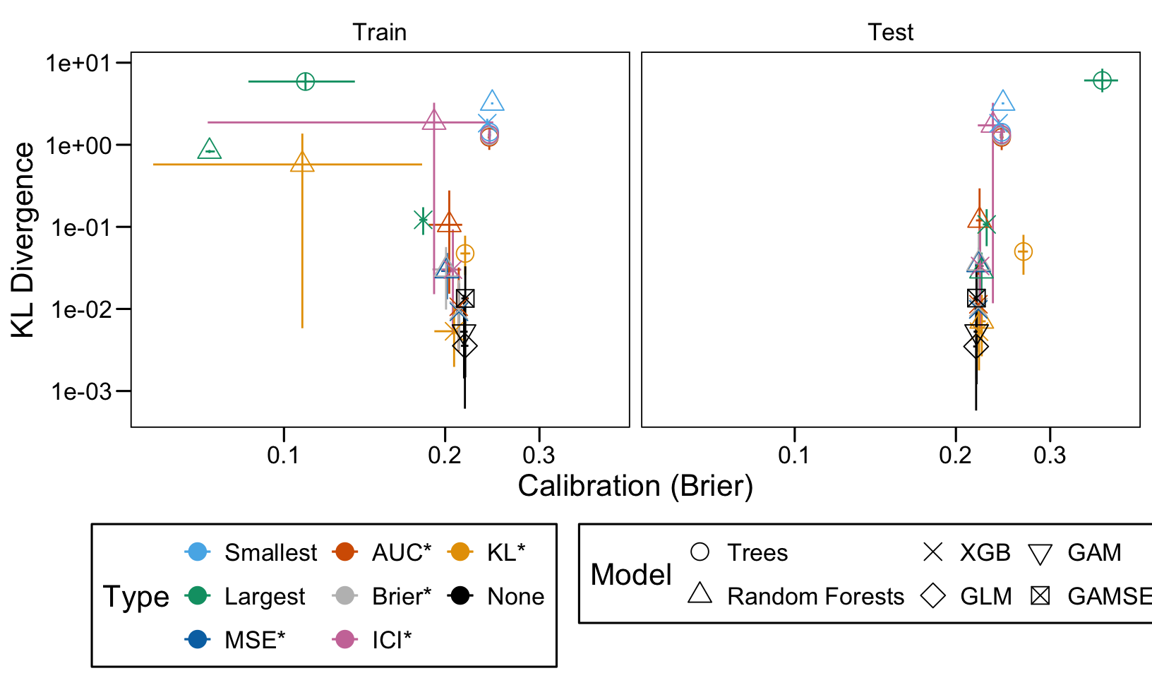
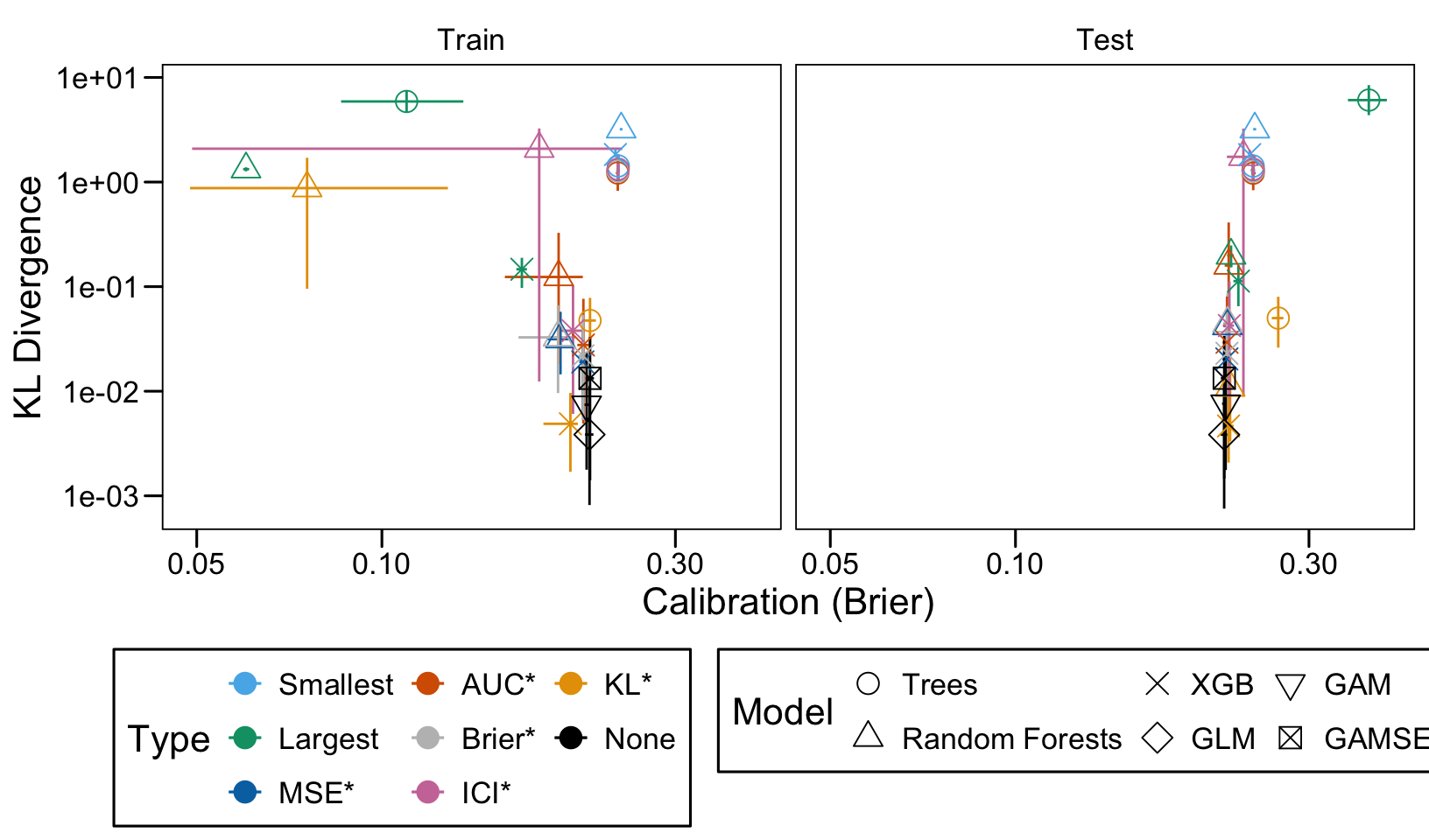
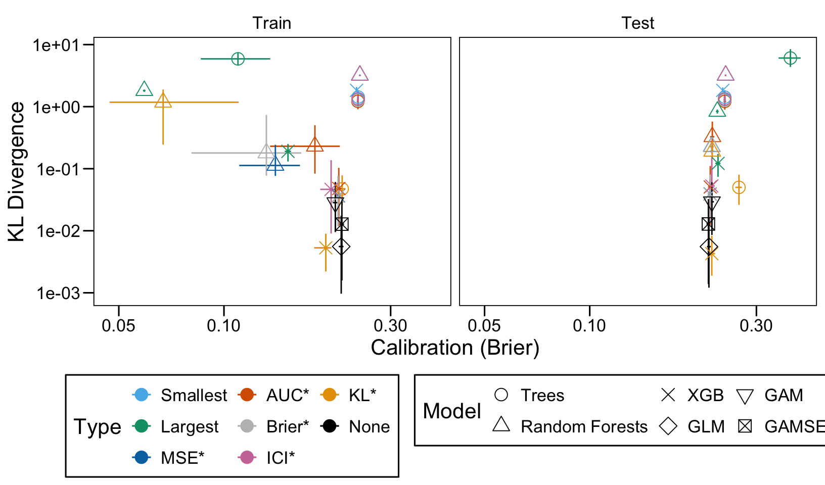
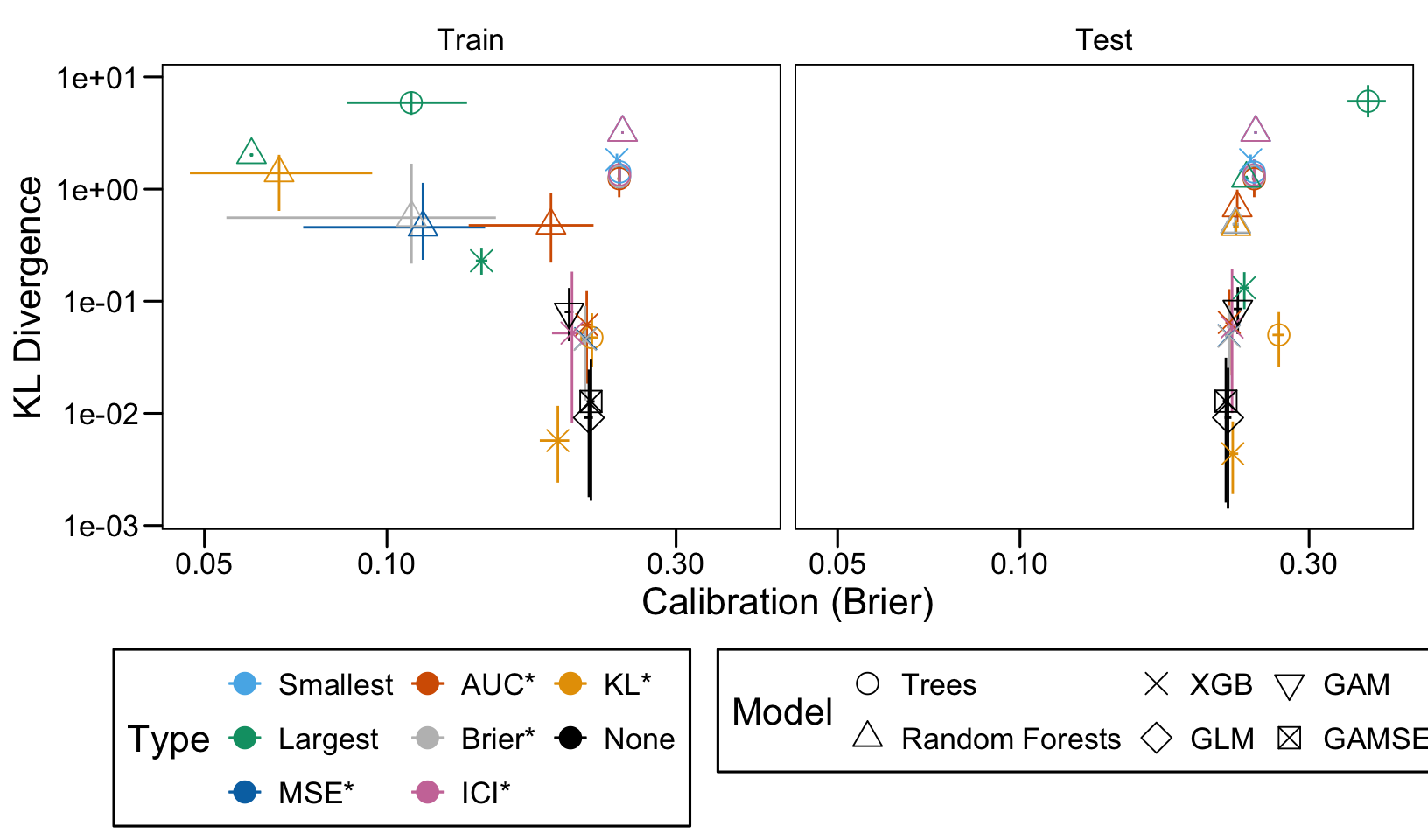
We define a function, plot_comparison() to plot the results. The left panel of the figure shows values computed on the train set, whereas the right panel shows values computed on the validation set. The shape of the dots represent the average of the metric computed over the 100 replications for the model of interest (smallest, largest, AUC*, MSE*, ICI*, KL*). The color of the points allows to identify the models of interest. Lastly, the vertical and horizontal segments show the 95% intervals computed over the 100 replications for the models of interest.

Code
plot_comparison <- function(scenario, calib_metric) {
  df_plot <- models_interest |> filter(scenario == !!scenario)
  model_shapes <- c(
    "Trees" = 1,
    "Random Forests" = 2,
    "XGB" = 4,
    "GLM" = 5,
    "GAM" = 6,
    "GAMSEL" = 7
  )
  model_shapes <- model_shapes[names(model_shapes) %in% df_plot$model]
  
  ggplot(
    data = df_plot,
    mapping = aes(
      colour = result_type,
      shape = model
    )
  ) +
    geom_segment(
      mapping = aes(
        x = !!sym(str_c(calib_metric, "_lower")),
        y = KL_20_true_probas,
        xend = !!sym(str_c(calib_metric, "_upper")),
        yend = KL_20_true_probas
      ),
      linetype = "solid",
      linewidth = .5
    ) +
    geom_segment(
      mapping = aes(
        x = !!sym(calib_metric), 
        y = KL_20_true_probas_lower,
        xend = !!sym(calib_metric), 
        yend = KL_20_true_probas_upper
      ),
      linetype = "solid",
      linewidth = .5
    ) +
    geom_point(
      mapping = aes(x = !!sym(calib_metric), y = KL_20_true_probas),
      size = 4
    ) +
    labs(
      x = str_c("Calibration (", ifelse(calib_metric == "ici", "ICI", "Brier"), ")"), 
      y = "KL Divergence"
    ) +
    scale_colour_manual("Type", values = colour_result_type) +
    scale_shape_manual(
      "Model", values = c(model_shapes)) +
    facet_wrap(~sample) +
    theme_paper() +
    scale_x_log10() +
    scale_y_log10() +
    guides(colour=guide_legend(ncol = 3))
}
Comparison of models (DGP 1, 0 noise variables)

Comparison of models (DGP 1, 10 noise variables)

Comparison of models (DGP 1, 50 noise variables)

Comparison of models (DGP 1, 100 noise variables)

Comparison of models (DGP 2, 0 noise variables)

Comparison of models (DGP 2, 10 noise variables)

Comparison of models (DGP 2, 50 noise variables)

Comparison of models (DGP 2, 100 noise variables)

Comparison of models (DGP 3, 0 noise variables)

Comparison of models (DGP 3, 10 noise variables)

Comparison of models (DGP 3, 50 noise variables)

Comparison of models (DGP 3, 100 noise variables)

Comparison of models (DGP 4, 0 noise variables)

Comparison of models (DGP 4, 10 noise variables)

Comparison of models (DGP 4, 50 noise variables)

Comparison of models (DGP 4, 100 noise variables)

14.1 Tables

We also visualize the results in tables. For each model within a given scenario, we report the average AUC, Brier Score, ICI, and KL divergence over 100 replications for the ‘best’ model. For ensemble tree models, the ‘best’ model is identified either when maximizing the AUC (denoted \(AUC^*\)), when minimizing the Brier Score (denoted \(Brier^*\)), the ICI (denoted \(ICI^*\)), or the KL divergence (denoted \(KL^*\)). When the best model is selected based anything but the AUC, we compute the variation in the metric as the difference between the metric obtained when minimizing either the Brier score, the ICI, or the KL divergence and the metric obtained when maximizing AUC. Thus, negative values indicate a decrease in the metric compared to when the best model is selected by optimizing AUC. For general linear models, the only metrics reported are the AUC, Brier, ICI, and KL divergence.

Display the codes to create the summary table.
table_models_interest_mean <- 
  models_interest |> 
  filter(sample == "Test") |> 
  select(
    scenario, sample, model, result_type, 
    AUC, brier, ici, kl = KL_20_true_probas, quant_ratio
  ) |> 
  filter(
    result_type %in% c("AUC*", "Brier*", "ICI*", "KL*", "None")
  ) |> 
  mutate(result_type = fct_recode(result_type, "KL*" = "None")) |> 
  mutate(value_type = "mean")

table_models_interest_sd <- 
  models_interest |> 
  filter(sample == "Test") |> 
  select(
    scenario, sample, model, result_type, 
    AUC = AUC_sd, brier = brier_sd, ici = ici_sd, kl = KL_20_true_probas_sd, quant_ratio = quant_ratio_sd
  ) |> 
  filter(
    result_type %in% c("AUC*", "Brier*", "ICI*", "KL*", "None")
  ) |> 
  mutate(result_type = fct_recode(result_type, "KL*" = "None")) |> 
  mutate(value_type = "sd")


red_colours <- c(
  "#FFD6D6", "#FFCCCC", "#FFC2C2", "#FFB8B8", "#FFADAD", 
  "#FFA3A3", "#FF9999", "#FF8F8F", "#FF8585", "#FF7A7A"
)
red_colours_txt <- c(
  "#333333", "#333333", "#2B2B2B", "#2B2B2B", "#232323", 
  "#1F1F1F", "#1A1A1A", "#141414", "#101010", "#0A0A0A"
)
green_colours <- c(
  "#E9F6E9", "#D4F2D4", "#BFEFBF", "#AADCA9", "#96C996",
  "#81B781", "#6CA56C", "#578252", "#426F42", "#2F5D2F"
)
green_colours_txt <- c(
  "#1A1A1A", "#1A1A1A", "#1A1A1A", "#1A1A1A", "#1A1A1A",
  "#E6E6E6", "#E6E6E6", "#E6E6E6", "#E6E6E6", "#E6E6E6"
)

accuracy_digits <- 0.01

table_kb <- 
  table_models_interest_mean |> 
  bind_rows(table_models_interest_sd) |> 
  pivot_wider(
    names_from = "result_type", 
    values_from = c("AUC", "brier", "ici", "kl", "quant_ratio")
  ) |> 
  mutate(
    value_type = factor(value_type, levels = c("mean", "sd")),
    scenario = factor(scenario)
  ) |> 
  select(
    scenario, model, value_type,
    # # columns for GLM/GAM/GAMSEL
    # AUC_None, ici_None, kl_None, 
    # columns for ML models selected based on AUC
    `AUC_AUC*`, `brier_AUC*`, `ici_AUC*`, `kl_AUC*`, `quant_ratio_AUC*`,
    # columns for ML models selected based on Brier score
    `AUC_Brier*`,  `brier_Brier*`, `ici_Brier*`, `kl_Brier*`, `quant_ratio_Brier*`,
    # columns for ML models selected based on ICI
    `AUC_ICI*`, `brier_ICI*`, `ici_ICI*`, `kl_ICI*`, `quant_ratio_ICI*`,
    # columns for ML models selected based on KL dist
    `AUC_KL*`, `brier_KL*`, `ici_KL*`, `kl_KL*`, `quant_ratio_KL*`
  ) |> 
  arrange(scenario, model, value_type) |> 
  mutate(
    # Difference in metrics computed when minnimizing Brier wrt when maximizing AUC
    diff_AUC_Brier = `AUC_Brier*` - `AUC_AUC*`,
    diff_brier_Brier = `brier_Brier*` - `brier_AUC*`,
    diff_ICI_Brier = `ici_Brier*` - `ici_AUC*`,
    diff_KL_Brier = `kl_Brier*` - `kl_AUC*`,
    diff_quant_ratio_Brier = `quant_ratio_Brier*` - `quant_ratio_AUC*`,
    # Difference in metrics computed when minnimizing ICI wrt when maximizing AUC
    diff_AUC_ICI = `AUC_ICI*` - `AUC_AUC*`,
    diff_brier_ICI = `brier_ICI*` - `brier_AUC*`,
    diff_ICI_ICI = `ici_ICI*` - `ici_AUC*`,
    diff_KL_ICI = `kl_ICI*` - `kl_AUC*`,
    diff_quant_ratio_ICI = `quant_ratio_ICI*` - `quant_ratio_AUC*`,
    # Difference in metrics computed when minnimizing KL wrt when maximizing AUC
    diff_AUC_KL = `AUC_KL*` - `AUC_AUC*`,
    diff_brier_KL = `brier_KL*` - `brier_AUC*`,
    diff_ICI_KL = `ici_KL*` - `ici_AUC*`,
    diff_KL_KL = `kl_KL*` - `kl_AUC*`,
    diff_quant_ratio_KL = `quant_ratio_KL*` - `quant_ratio_AUC*`
  ) |> 
  ungroup()

get_range_for_colours <- function(variable_name) {
  value <- table_kb |> 
    filter(value_type == "mean") |> 
    pull(!!variable_name) |> 
    range(na.rm = TRUE) |> abs() |> max()
  value * c(-1, 1)
}

get_colour <- function(variable, value_type, min_or_max, colour_type) {
  if (value_type == "mean") {
    variable_string <- deparse(substitute(variable))
    if (colour_type == "bg") {
      # background colour
      if (min_or_max == "min") {
        colours <- rev(c(rev(red_colours), green_colours))
      } else {
        colours <- c(rev(red_colours), rev(green_colours))
      }
    } else {
      # text colour
      if (min_or_max == "min") {
        colours <- rev(c(rev(red_colours_txt), green_colours_txt))
      } else {
        colours <- c(rev(red_colours_txt), rev(green_colours_txt))
      }
    }
    res <- kableExtra::spec_color(
      variable,
      palette = colours,
      scale_from = get_range_for_colours(variable_string),
      na_color = "white"
    )
  } else {
    res <- "white"
  }
  res
}

table_kb <- 
  table_kb |> 
  rowwise() |> 
  mutate(
    # Difference in metrics computed when minnimizing ICI wrt when maximizing AUC
    diff_AUC_Brier_bgcol = get_colour(diff_AUC_Brier, value_type, "max", "bg"),
    diff_AUC_Brier_txtcol = get_colour(diff_AUC_Brier, value_type, "max", "txt"),
    diff_brier_Brier_bgcol = get_colour(diff_brier_Brier, value_type, "min", "bg"),
    diff_brier_Brier_txtcol = get_colour(diff_brier_Brier, value_type, "min", "txt"),
    diff_ICI_Brier_bgcol = get_colour(diff_ICI_Brier, value_type, "min", "bg"),
    diff_ICI_Brier_txtcol = get_colour(diff_ICI_Brier, value_type, "min", "txt"),
    diff_KL_Brier_bgcol = get_colour(diff_KL_Brier, value_type, "min", "bg"),
    diff_KL_Brier_txtcol = get_colour(diff_KL_Brier, value_type, "min", "txt"),
    diff_quant_ratio_Brier_bgcol = get_colour(diff_quant_ratio_Brier, value_type, "min", "bg"),
    diff_quant_ratio_Brier_txtcol = get_colour(diff_quant_ratio_Brier, value_type, "min", "txt"),
    # Difference in metrics computed when minnimizing ICI wrt when maximizing AUC
    diff_AUC_ICI_bgcol = get_colour(diff_AUC_ICI, value_type, "max", "bg"),
    diff_AUC_ICI_txtcol = get_colour(diff_AUC_ICI, value_type, "max", "txt"),
    diff_brier_ICI_bgcol = get_colour(diff_brier_ICI, value_type, "min", "bg"),
    diff_brier_ICI_txtcol = get_colour(diff_brier_ICI, value_type, "min", "txt"),
    diff_ICI_ICI_bgcol = get_colour(diff_ICI_ICI, value_type, "min", "bg"),
    diff_ICI_ICI_txtcol = get_colour(diff_ICI_ICI, value_type, "min", "txt"),
    diff_KL_ICI_bgcol = get_colour(diff_KL_ICI, value_type, "min", "bg"),
    diff_KL_ICI_txtcol = get_colour(diff_KL_ICI, value_type, "min", "txt"),
    diff_quant_ratio_ICI_bgcol = get_colour(diff_quant_ratio_ICI, value_type, "min", "bg"),
    diff_quant_ratio_ICI_txtcol = get_colour(diff_quant_ratio_ICI, value_type, "min", "txt"),
    # Difference in metrics computed when minnimizing KL wrt when maximizing AUC
    diff_AUC_KL_bgcol = get_colour(diff_AUC_KL, value_type, "max", "bg"),
    diff_AUC_KL_txtcol = get_colour(diff_AUC_KL, value_type, "max", "txt"),
    diff_brier_KL_bgcol = get_colour(diff_brier_KL, value_type, "min", "bg"),
    diff_brier_KL_txtcol = get_colour(diff_brier_KL, value_type, "min", "txt"),
    diff_ICI_KL_bgcol = get_colour(diff_ICI_KL, value_type, "min", "bg"),
    diff_ICI_KL_txtcol = get_colour(diff_ICI_KL, value_type, "min", "txt"),
    diff_KL_KL_bgcol = get_colour(diff_KL_KL, value_type, "min", "bg"),
    diff_KL_KL_txtcol = get_colour(diff_KL_KL, value_type, "min", "txt"),
    diff_quant_ratio_KL_bgcol = get_colour(diff_quant_ratio_KL, value_type, "min", "bg"),
    diff_quant_ratio_KL_txtcol = get_colour(diff_quant_ratio_KL, value_type, "min", "txt")
  ) |> 
  mutate(
    across(
      where(is.numeric), 
      ~ifelse(value_type == "mean", 
              scales::number(.x, accuracy = accuracy_digits),
              str_c("(", scales::number(.x, accuracy = accuracy_digits), ")")
      )
    )
  )


opts <- options(knitr.kable.NA = "")


print_table <- function(scenario) {
  
  table_kb <- table_kb |> filter(scenario == !!scenario) |> 
    select(
      scenario, model,
      # Max AUC
      `AUC_AUC*`, `brier_AUC*`, `ici_AUC*`, `kl_AUC*`, `quant_ratio_AUC*`,
      # Min Brier
      `AUC_Brier*`, `brier_Brier*`, `ici_Brier*`, `kl_Brier*`, `quant_ratio_Brier*`,
      diff_AUC_Brier, diff_brier_Brier, diff_ICI_Brier, diff_KL_Brier, diff_quant_ratio_Brier,
      # Min ICI
      `AUC_ICI*`, `brier_ICI*`, `ici_ICI*`, `kl_ICI*`, `quant_ratio_ICI*`,
      diff_AUC_ICI, diff_brier_ICI, diff_ICI_ICI, diff_KL_ICI, diff_quant_ratio_ICI,
      # Min KL
      `AUC_KL*`, `brier_KL*`, `ici_KL*`, `kl_KL*`, `quant_ratio_KL*`,
      diff_AUC_KL, diff_brier_KL, diff_ICI_KL, diff_KL_KL, diff_quant_ratio_KL,
      # colouring variables
      diff_AUC_Brier_bgcol, diff_brier_Brier_bgcol, diff_ICI_Brier_bgcol, diff_KL_Brier_bgcol, diff_quant_ratio_Brier_bgcol,
      #
      diff_AUC_Brier_txtcol, diff_brier_Brier_txtcol, diff_ICI_Brier_txtcol, diff_KL_Brier_txtcol, diff_quant_ratio_Brier_txtcol,
      #
      diff_AUC_ICI_bgcol, diff_brier_ICI_bgcol, diff_ICI_ICI_bgcol, diff_KL_ICI_bgcol, diff_quant_ratio_ICI_bgcol,
      #
      diff_AUC_ICI_txtcol, diff_brier_ICI_txtcol, diff_ICI_ICI_txtcol, diff_KL_ICI_txtcol, diff_quant_ratio_ICI_txtcol,
      #
      diff_AUC_KL_bgcol, diff_brier_KL_bgcol, diff_ICI_KL_bgcol, diff_KL_KL_bgcol, diff_quant_ratio_KL_bgcol,
      #
      diff_AUC_KL_txtcol, diff_brier_KL_txtcol, diff_ICI_KL_txtcol, diff_KL_KL_txtcol, diff_quant_ratio_KL_txtcol
    )
  
  knitr::kable(
    table_kb |> 
      select(
        scenario, model,
        # Max AUC
        `AUC_AUC*`, `brier_AUC*`, `ici_AUC*`, `kl_AUC*`, `quant_ratio_AUC*`,
        # Min Brier
        `AUC_Brier*`, `brier_Brier*`, `ici_Brier*`, `kl_Brier*`, `quant_ratio_Brier*`,
        diff_AUC_Brier, diff_brier_Brier, diff_ICI_Brier, diff_KL_Brier, diff_quant_ratio_Brier,
        # Min ICI
        `AUC_ICI*`, `brier_ICI*`, `ici_ICI*`, `kl_ICI*`, `quant_ratio_ICI*`, 
        diff_AUC_ICI, diff_brier_ICI, diff_ICI_ICI, diff_KL_ICI, diff_quant_ratio_ICI,
        # Min KL
        `AUC_KL*`, `brier_KL*`, `ici_KL*`, `kl_KL*`, `quant_ratio_KL*`,
        diff_AUC_KL, diff_brier_KL, diff_ICI_KL, diff_KL_KL, diff_quant_ratio_KL
      ),
    col.names = c(
      "Scenario", "Model",
      # # columns for GLM/GAM/GAMSEL
      # "AUC", "ICI", "KL", 
      # columns for ML models selected based on AUC
      "AUC", "Brier", "ICI", "KL", "Quant. Ratio",
      # columns for ML models selected based on Brier
      "AUC", "Brier", "ICI", "KL", "Quant. Ratio", "ΔAUC", "ΔBrier", "ΔICI", "ΔKL", "ΔQR",
      # columns for ML models selected based on ICI
      "AUC", "Brier", "ICI", "KL", "Quant. Ratio", "ΔAUC", "ΔBrier", "ΔICI", "ΔKL", "ΔQR",
      # columns for ML models selected based on KL dist
      "AUC", "Brier", "ICI", "KL", "Quant. Ratio", "ΔAUC", "ΔBrier","ΔICI", "ΔKL", "ΔQR"
    ),
    align = str_c("cl", str_c(rep("c", 5+10*3), collapse = ""), collapse = ""),
    escape = FALSE, booktabs = T, digits = 3, format = "markdown") |> 
    # Difference in metrics computed when minnimizing Brier wrt when maximizing AUC
    kableExtra::column_spec(
      which(colnames(table_kb) == "diff_AUC_Brier"),
      background = table_kb$diff_AUC_Brier_bgcol,
      color = table_kb$diff_AUC_Brier_txtcol
    ) |>
    kableExtra::column_spec(
      which(colnames(table_kb) == "diff_brier_Brier"),
      background = table_kb$diff_brier_Brier_bgcol,
      color = table_kb$diff_brier_Brier_txtcol
    ) |>
    kableExtra::column_spec(
      which(colnames(table_kb) == "diff_ICI_Brier"),
      background = table_kb$diff_ICI_Brier_bgcol,
      color = table_kb$diff_ICI_Brier_txtcol
    ) |>
    kableExtra::column_spec(
      which(colnames(table_kb) == "diff_KL_Brier"),
      background = table_kb$diff_KL_Brier_bgcol,
      color = table_kb$diff_KL_Brier_txtcol
    ) |>
    kableExtra::column_spec(
      which(colnames(table_kb) == "diff_quant_ratio_Brier"),
      background = table_kb$diff_quant_ratio_Brier_bgcol,
      color = table_kb$diff_quant_ratio_Brier_txtcol
    ) |>
    # Difference in metrics computed when minnimizing ICI wrt when maximizing AUC
    kableExtra::column_spec(
      which(colnames(table_kb) == "diff_AUC_ICI"),
      background = table_kb$diff_AUC_ICI_bgcol,
      color = table_kb$diff_AUC_ICI_txtcol
    ) |>
    kableExtra::column_spec(
      which(colnames(table_kb) == "diff_brier_ICI"),
      background = table_kb$diff_brier_ICI_bgcol,
      color = table_kb$diff_brier_ICI_txtcol
    ) |>
    kableExtra::column_spec(
      which(colnames(table_kb) == "diff_ICI_ICI"),
      background = table_kb$diff_ICI_ICI_bgcol,
      color = table_kb$diff_ICI_ICI_txtcol
    ) |>
    kableExtra::column_spec(
      which(colnames(table_kb) == "diff_KL_ICI"),
      background = table_kb$diff_KL_ICI_bgcol,
      color = table_kb$diff_KL_ICI_txtcol
    ) |>
    kableExtra::column_spec(
      which(colnames(table_kb) == "diff_quant_ratio_ICI"),
      background = table_kb$diff_quant_ratio_ICI_bgcol,
      color = table_kb$diff_quant_ratio_ICI_txtcol
    ) |>
    # Difference in metrics computed when minnimizing KL wrt when maximizing AUC
    kableExtra::column_spec(
      which(colnames(table_kb) == "diff_AUC_KL"),
      background = table_kb$diff_AUC_KL_bgcol,
      color = table_kb$diff_AUC_KL_txtcol
    ) |>
    kableExtra::column_spec(
      which(colnames(table_kb) == "diff_brier_KL"),
      background = table_kb$diff_brier_KL_bgcol,
      color = table_kb$diff_brier_KL_txtcol
    ) |>
    kableExtra::column_spec(
      which(colnames(table_kb) == "diff_ICI_KL"),
      background = table_kb$diff_ICI_KL_bgcol,
      color = table_kb$diff_ICI_KL_txtcol
    ) |>
    kableExtra::column_spec(
      which(colnames(table_kb) == "diff_KL_KL"),
      background = table_kb$diff_KL_KL_bgcol,
      color = table_kb$diff_KL_KL_txtcol
    ) |>
     kableExtra::column_spec(
      which(colnames(table_kb) == "diff_quant_ratio_KL"),
      background = table_kb$diff_quant_ratio_KL_bgcol,
      color = table_kb$diff_quant_ratio_KL_txtcol
    ) |>
    kableExtra::collapse_rows(columns = 1:2, valign = "top") |>
    kableExtra::add_header_above(
      c(" " = 2,
        # "Generalized Lin. Models" = 3,
        "AUC*" = 5,
        "Brier*" = 10,
        "ICI*" = 10,
        "KL*" = 10
      )
    )
}
AUC*
Brier*
ICI*
KL*
Scenario Model AUC Brier ICI KL Quant. Ratio AUC Brier ICI KL Quant. Ratio ΔAUC ΔBrier ΔICI ΔKL ΔQR AUC Brier ICI KL Quant. Ratio ΔAUC ΔBrier ΔICI ΔKL ΔQR AUC Brier ICI KL Quant. Ratio ΔAUC ΔBrier ΔICI ΔKL ΔQR
1 Trees 0.75 0.20 0.01 0.28 1.02 0.75 0.20 0.01 0.28 1.02 0.00 0.00 0.00 0.00 0.00 0.73 0.21 0.01 1.26 0.98 -0.02 0.00 0.00 0.98 -0.05 0.74 0.21 0.03 0.09 1.08 -0.01 0.00 0.01 -0.20 0.06
(0.01) (0.00) (0.00) (0.12) (0.05) (0.01) (0.00) (0.00) (0.13) (0.05) (0.00) (0.00) (0.00) (0.01) (0.00) (0.01) (0.00) (0.00) (0.54) (0.08) (0.01) (0.00) (0.00) (0.43) (0.03) (0.01) (0.00) (0.01) (0.02) (0.04) (0.00) (0.00) (0.01) (-0.10) (-0.01)
Random Forests 0.76 0.20 0.01 0.06 1.00 0.76 0.20 0.01 0.05 1.00 0.00 0.00 0.00 0.00 0.00 0.59 0.23 0.01 2.61 0.32 -0.17 0.03 0.00 2.55 -0.67 0.75 0.20 0.02 0.03 1.04 -0.01 0.00 0.01 -0.03 0.04
(0.00) (0.00) (0.00) (0.02) (0.03) (0.00) (0.00) (0.00) (0.02) (0.03) (0.00) (0.00) (0.00) (0.00) (0.00) (0.12) (0.02) (0.00) (1.75) (0.46) (0.11) (0.02) (0.00) (1.73) (0.43) (0.01) (0.00) (0.01) (0.01) (0.02) (0.00) (0.00) (0.00) (-0.01) (0.00)
XGB 0.76 0.20 0.01 0.05 0.96 0.76 0.20 0.01 0.04 0.97 0.00 0.00 0.00 -0.01 0.01 0.75 0.20 0.01 0.05 0.97 0.00 0.00 0.00 -0.01 0.01 0.75 0.20 0.01 0.02 1.01 0.00 0.00 0.00 -0.03 0.04
(0.00) (0.00) (0.00) (0.03) (0.03) (0.00) (0.00) (0.00) (0.02) (0.02) (0.00) (0.00) (0.00) (-0.01) (-0.01) (0.01) (0.00) (0.00) (0.02) (0.03) (0.00) (0.00) (0.00) (-0.01) (0.00) (0.01) (0.00) (0.00) (0.01) (0.02) (0.00) (0.00) (0.00) (-0.02) (-0.01)
GLM 0.76 0.20 0.01 0.00 1.00
(0.01) (0.00) (0.00) (0.00) (0.02)
GAM 0.76 0.20 0.01 0.00 1.00
(0.01) (0.00) (0.00) (0.00) (0.02)
GAMSEL 0.76 0.20 0.01 0.01 0.93
(0.00) (0.00) (0.00) (0.01) (0.02)

Comparison of metrics for models chosen based on AUC, on Brier Score, on ICI, or on KL divergence (DGP 1, 0 noise variables)

AUC*
Brier*
ICI*
KL*
Scenario Model AUC Brier ICI KL Quant. Ratio AUC Brier ICI KL Quant. Ratio ΔAUC ΔBrier ΔICI ΔKL ΔQR AUC Brier ICI KL Quant. Ratio ΔAUC ΔBrier ΔICI ΔKL ΔQR AUC Brier ICI KL Quant. Ratio ΔAUC ΔBrier ΔICI ΔKL ΔQR
2 Trees 0.75 0.20 0.01 0.27 1.02 0.75 0.20 0.01 0.29 1.02 0.00 0.00 0.00 0.01 0.00 0.73 0.21 0.01 1.22 0.98 -0.02 0.00 0.00 0.95 -0.04 0.74 0.21 0.03 0.09 1.08 -0.01 0.00 0.01 -0.19 0.06
(0.01) (0.00) (0.00) (0.12) (0.05) (0.01) (0.00) (0.00) (0.13) (0.05) (0.00) (0.00) (0.00) (0.01) (0.00) (0.01) (0.00) (0.00) (0.56) (0.08) (0.01) (0.00) (0.00) (0.44) (0.03) (0.01) (0.00) (0.01) (0.02) (0.04) (0.00) (0.00) (0.01) (-0.10) (-0.01)
Random Forests 0.76 0.20 0.01 0.06 0.98 0.75 0.20 0.01 0.05 0.98 0.00 0.00 0.00 -0.01 0.00 0.61 0.23 0.01 2.26 0.40 -0.15 0.03 0.00 2.21 -0.58 0.75 0.20 0.01 0.01 1.00 -0.01 0.00 0.00 -0.05 0.02
(0.00) (0.00) (0.00) (0.03) (0.03) (0.00) (0.00) (0.00) (0.02) (0.03) (0.00) (0.00) (0.00) (-0.01) (-0.01) (0.12) (0.02) (0.00) (1.87) (0.48) (0.12) (0.02) (0.00) (1.84) (0.45) (0.01) (0.00) (0.00) (0.00) (0.02) (0.00) (0.00) (0.00) (-0.02) (-0.01)
XGB 0.76 0.20 0.01 0.07 0.93 0.76 0.20 0.01 0.05 0.95 0.00 0.00 0.00 -0.02 0.01 0.75 0.20 0.01 0.03 0.97 -0.01 0.00 0.00 -0.03 0.03 0.75 0.20 0.02 0.01 1.02 -0.01 0.00 0.00 -0.06 0.08
(0.00) (0.00) (0.01) (0.05) (0.04) (0.00) (0.00) (0.00) (0.02) (0.02) (0.00) (0.00) (0.00) (-0.02) (-0.01) (0.01) (0.00) (0.00) (0.02) (0.03) (0.00) (0.00) (0.00) (-0.03) (-0.01) (0.01) (0.00) (0.00) (0.00) (0.02) (0.00) (0.00) (0.00) (-0.04) (-0.02)
GLM 0.76 0.20 0.01 0.00 1.00
(0.01) (0.00) (0.00) (0.00) (0.02)
GAM 0.76 0.20 0.01 0.00 1.01
(0.01) (0.00) (0.00) (0.00) (0.02)
GAMSEL 0.76 0.20 0.01 0.01 0.93
(0.01) (0.00) (0.00) (0.01) (0.02)

Comparison of metrics for models chosen based on AUC, on Brier Score, on ICI, or on KL divergence (DGP 1, 10 noise variables)

AUC*
Brier*
ICI*
KL*
Scenario Model AUC Brier ICI KL Quant. Ratio AUC Brier ICI KL Quant. Ratio ΔAUC ΔBrier ΔICI ΔKL ΔQR AUC Brier ICI KL Quant. Ratio ΔAUC ΔBrier ΔICI ΔKL ΔQR AUC Brier ICI KL Quant. Ratio ΔAUC ΔBrier ΔICI ΔKL ΔQR
3 Trees 0.75 0.20 0.01 0.27 1.02 0.75 0.20 0.01 0.28 1.02 0.00 0.00 0.00 0.01 0.00 0.73 0.21 0.01 1.23 0.98 -0.02 0.00 0.00 0.96 -0.05 0.74 0.21 0.03 0.09 1.08 -0.01 0.00 0.01 -0.19 0.06
(0.01) (0.00) (0.00) (0.12) (0.05) (0.01) (0.00) (0.00) (0.13) (0.05) (0.00) (0.00) (0.00) (0.01) (0.00) (0.01) (0.00) (0.00) (0.55) (0.08) (0.01) (0.00) (0.00) (0.44) (0.03) (0.01) (0.00) (0.01) (0.02) (0.04) (0.00) (0.00) (0.01) (-0.10) (-0.01)
Random Forests 0.75 0.20 0.04 0.27 0.76 0.75 0.20 0.03 0.20 0.80 0.00 0.00 -0.01 -0.07 0.04 0.50 0.25 0.01 3.82 0.00 -0.25 0.05 -0.03 3.56 -0.76 0.75 0.21 0.03 0.14 0.81 0.00 0.00 -0.01 -0.12 0.04
(0.00) (0.00) (0.01) (0.05) (0.03) (0.01) (0.00) (0.01) (0.03) (0.02) (0.00) (0.00) (0.00) (-0.02) (-0.01) (0.00) (0.00) (0.00) (0.05) (0.00) (0.00) (0.00) (0.00) (0.00) (-0.03) (0.01) (0.00) (0.01) (0.02) (0.02) (0.00) (0.00) (0.00) (-0.04) (-0.01)
XGB 0.76 0.20 0.02 0.09 0.91 0.76 0.20 0.01 0.06 0.93 0.00 0.00 0.00 -0.02 0.02 0.75 0.20 0.01 0.04 0.96 -0.01 0.00 -0.01 -0.05 0.05 0.74 0.21 0.02 0.01 1.02 -0.01 0.00 0.00 -0.08 0.10
(0.00) (0.00) (0.01) (0.05) (0.04) (0.00) (0.00) (0.00) (0.03) (0.02) (0.00) (0.00) (0.00) (-0.02) (-0.01) (0.01) (0.00) (0.00) (0.02) (0.03) (0.00) (0.00) (0.00) (-0.02) (-0.01) (0.01) (0.00) (0.01) (0.00) (0.02) (0.00) (0.00) (0.00) (-0.04) (-0.02)
GLM 0.76 0.20 0.01 0.00 1.01
(0.01) (0.00) (0.00) (0.00) (0.02)
GAM 0.75 0.20 0.02 0.01 1.05
(0.01) (0.00) (0.01) (0.01) (0.02)
GAMSEL 0.76 0.20 0.01 0.01 0.93
(0.01) (0.00) (0.00) (0.01) (0.02)

Comparison of metrics for models chosen based on AUC, on Brier Score, on ICI, or on KL divergence (DGP 1, 50 noise variables)

AUC*
Brier*
ICI*
KL*
Scenario Model AUC Brier ICI KL Quant. Ratio AUC Brier ICI KL Quant. Ratio ΔAUC ΔBrier ΔICI ΔKL ΔQR AUC Brier ICI KL Quant. Ratio ΔAUC ΔBrier ΔICI ΔKL ΔQR AUC Brier ICI KL Quant. Ratio ΔAUC ΔBrier ΔICI ΔKL ΔQR
4 Trees 0.75 0.20 0.01 0.28 1.02 0.75 0.20 0.01 0.29 1.02 0.00 0.00 0.00 0.01 0.00 0.73 0.21 0.01 1.22 0.98 -0.02 0.00 0.00 0.94 -0.05 0.74 0.21 0.03 0.09 1.08 -0.01 0.00 0.01 -0.19 0.05
(0.01) (0.00) (0.00) (0.12) (0.05) (0.01) (0.00) (0.00) (0.13) (0.05) (0.00) (0.00) (0.00) (0.01) (0.00) (0.01) (0.00) (0.00) (0.54) (0.08) (0.01) (0.00) (0.00) (0.42) (0.03) (0.01) (0.00) (0.01) (0.02) (0.04) (0.00) (0.00) (0.00) (-0.10) (-0.01)
Random Forests 0.75 0.21 0.07 0.59 0.57 0.74 0.21 0.06 0.47 0.61 0.00 0.00 -0.01 -0.11 0.04 0.50 0.25 0.01 3.82 0.00 -0.24 0.04 -0.06 3.23 -0.57 0.74 0.21 0.06 0.45 0.61 0.00 0.00 -0.01 -0.13 0.04
(0.00) (0.00) (0.01) (0.08) (0.03) (0.01) (0.00) (0.01) (0.03) (0.02) (0.00) (0.00) (0.00) (-0.04) (-0.01) (0.00) (0.00) (0.00) (0.05) (0.00) (0.00) (0.00) (0.00) (-0.02) (-0.03) (0.01) (0.00) (0.01) (0.03) (0.02) (0.00) (0.00) (0.00) (-0.05) (-0.01)
XGB 0.76 0.20 0.02 0.09 0.91 0.76 0.20 0.01 0.07 0.92 0.00 0.00 0.00 -0.02 0.01 0.75 0.20 0.01 0.04 0.96 -0.01 0.00 -0.01 -0.05 0.05 0.74 0.21 0.02 0.01 1.02 -0.01 0.00 0.00 -0.08 0.11
(0.00) (0.00) (0.01) (0.04) (0.03) (0.00) (0.00) (0.00) (0.03) (0.03) (0.00) (0.00) (0.00) (-0.01) (-0.01) (0.01) (0.00) (0.00) (0.02) (0.02) (0.00) (0.00) (0.00) (-0.02) (-0.01) (0.01) (0.00) (0.01) (0.00) (0.01) (0.00) (0.00) (0.00) (-0.03) (-0.02)
GLM 0.75 0.20 0.01 0.00 1.02
(0.01) (0.00) (0.00) (0.00) (0.02)
GAM 0.74 0.21 0.04 0.03 1.10
(0.01) (0.00) (0.00) (0.01) (0.02)
GAMSEL 0.76 0.20 0.01 0.01 0.93
(0.01) (0.00) (0.00) (0.01) (0.02)

Comparison of metrics for models chosen based on AUC, on Brier Score, on ICI, or on KL divergence (DGP 1, 100 noise variables)

AUC*
Brier*
ICI*
KL*
Scenario Model AUC Brier ICI KL Quant. Ratio AUC Brier ICI KL Quant. Ratio ΔAUC ΔBrier ΔICI ΔKL ΔQR AUC Brier ICI KL Quant. Ratio ΔAUC ΔBrier ΔICI ΔKL ΔQR AUC Brier ICI KL Quant. Ratio ΔAUC ΔBrier ΔICI ΔKL ΔQR
5 Trees 0.83 0.12 0.01 0.24 1.03 0.83 0.12 0.01 0.23 1.03 0.00 0.00 0.00 -0.01 0.00 0.81 0.13 0.01 0.84 0.97 -0.02 0.01 0.00 0.60 -0.06 0.82 0.13 0.03 0.06 1.07 -0.02 0.00 0.02 -0.18 0.04
(0.00) (0.00) (0.00) (0.10) (0.06) (0.00) (0.00) (0.00) (0.10) (0.05) (0.00) (0.00) (0.00) (0.00) (0.00) (0.02) (0.00) (0.00) (0.39) (0.13) (0.01) (0.00) (0.00) (0.29) (0.07) (0.01) (0.00) (0.01) (0.02) (0.04) (0.00) (0.00) (0.01) (-0.08) (-0.02)
Random Forests 0.84 0.12 0.01 0.04 1.01 0.84 0.12 0.01 0.04 1.01 0.00 0.00 0.00 -0.01 0.00 0.62 0.15 0.01 2.66 0.34 -0.22 0.03 0.00 2.62 -0.67 0.83 0.12 0.01 0.02 1.03 -0.01 0.00 0.00 -0.03 0.02
(0.00) (0.00) (0.00) (0.02) (0.03) (0.00) (0.00) (0.00) (0.01) (0.03) (0.00) (0.00) (0.00) (0.00) (0.00) (0.15) (0.02) (0.00) (1.70) (0.45) (0.15) (0.02) (0.00) (1.68) (0.42) (0.01) (0.00) (0.00) (0.01) (0.03) (0.00) (0.00) (0.00) (-0.01) (0.00)
XGB 0.84 0.12 0.01 0.03 0.99 0.84 0.12 0.01 0.03 0.99 0.00 0.00 0.00 0.00 0.00 0.84 0.12 0.01 0.02 1.00 0.00 0.00 0.00 0.00 0.01 0.84 0.12 0.01 0.01 1.01 0.00 0.00 0.00 -0.01 0.02
(0.00) (0.00) (0.00) (0.01) (0.03) (0.00) (0.00) (0.00) (0.01) (0.03) (0.00) (0.00) (0.00) (0.00) (0.00) (0.01) (0.00) (0.00) (0.01) (0.03) (0.00) (0.00) (0.00) (0.00) (0.00) (0.01) (0.00) (0.00) (0.01) (0.03) (0.00) (0.00) (0.00) (-0.01) (0.00)
GLM 0.84 0.12 0.01 0.02 0.99
(0.00) (0.00) (0.00) (0.00) (0.02)
GAM 0.84 0.12 0.01 0.01 1.00
(0.00) (0.00) (0.00) (0.00) (0.02)
GAMSEL 0.84 0.12 0.02 0.04 0.92
(0.00) (0.00) (0.00) (0.01) (0.02)

Comparison of metrics for models chosen based on AUC, on Brier Score, on ICI, or on KL divergence (DGP 2, 0 noise variables)

AUC*
Brier*
ICI*
KL*
Scenario Model AUC Brier ICI KL Quant. Ratio AUC Brier ICI KL Quant. Ratio ΔAUC ΔBrier ΔICI ΔKL ΔQR AUC Brier ICI KL Quant. Ratio ΔAUC ΔBrier ΔICI ΔKL ΔQR AUC Brier ICI KL Quant. Ratio ΔAUC ΔBrier ΔICI ΔKL ΔQR
6 Trees 0.83 0.12 0.01 0.24 1.03 0.83 0.12 0.01 0.23 1.03 0.00 0.00 0.00 -0.02 0.00 0.81 0.13 0.01 0.82 0.97 -0.02 0.01 0.00 0.58 -0.06 0.82 0.13 0.03 0.06 1.07 -0.02 0.00 0.02 -0.18 0.04
(0.00) (0.00) (0.00) (0.10) (0.06) (0.00) (0.00) (0.00) (0.10) (0.05) (0.00) (0.00) (0.00) (0.00) (0.00) (0.02) (0.00) (0.00) (0.39) (0.13) (0.01) (0.00) (0.00) (0.30) (0.07) (0.01) (0.00) (0.01) (0.02) (0.04) (0.00) (0.00) (0.01) (-0.08) (-0.02)
Random Forests 0.84 0.12 0.01 0.04 0.99 0.84 0.12 0.01 0.03 1.00 0.00 0.00 0.00 -0.01 0.00 0.61 0.15 0.01 2.65 0.32 -0.23 0.03 0.00 2.61 -0.68 0.83 0.12 0.01 0.01 1.00 -0.01 0.00 0.00 -0.03 0.01
(0.00) (0.00) (0.00) (0.01) (0.03) (0.00) (0.00) (0.00) (0.01) (0.03) (0.00) (0.00) (0.00) (0.00) (0.00) (0.15) (0.02) (0.00) (1.81) (0.46) (0.15) (0.02) (0.00) (1.80) (0.44) (0.01) (0.00) (0.00) (0.00) (0.03) (0.00) (0.00) (0.00) (-0.01) (0.00)
XGB 0.84 0.12 0.01 0.03 0.96 0.84 0.12 0.01 0.03 0.97 0.00 0.00 0.00 0.00 0.00 0.84 0.12 0.01 0.01 0.99 0.00 0.00 0.00 -0.02 0.02 0.83 0.12 0.01 0.01 1.00 -0.01 0.00 0.00 -0.02 0.04
(0.00) (0.00) (0.00) (0.01) (0.03) (0.00) (0.00) (0.00) (0.01) (0.03) (0.00) (0.00) (0.00) (0.00) (0.00) (0.01) (0.00) (0.00) (0.01) (0.03) (0.00) (0.00) (0.00) (-0.01) (0.00) (0.01) (0.00) (0.00) (0.00) (0.02) (0.00) (0.00) (0.00) (-0.01) (-0.01)
GLM 0.84 0.12 0.01 0.02 0.99
(0.01) (0.00) (0.00) (0.00) (0.02)
GAM 0.84 0.12 0.01 0.01 1.00
(0.01) (0.00) (0.00) (0.00) (0.02)
GAMSEL 0.84 0.12 0.02 0.04 0.92
(0.00) (0.00) (0.00) (0.01) (0.02)

Comparison of metrics for models chosen based on AUC, on Brier Score, on ICI, or on KL divergence (DGP 2, 10 noise variables)

AUC*
Brier*
ICI*
KL*
Scenario Model AUC Brier ICI KL Quant. Ratio AUC Brier ICI KL Quant. Ratio ΔAUC ΔBrier ΔICI ΔKL ΔQR AUC Brier ICI KL Quant. Ratio ΔAUC ΔBrier ΔICI ΔKL ΔQR AUC Brier ICI KL Quant. Ratio ΔAUC ΔBrier ΔICI ΔKL ΔQR
7 Trees 0.83 0.12 0.01 0.24 1.03 0.83 0.12 0.01 0.22 1.03 0.00 0.00 0.00 -0.02 -0.01 0.81 0.13 0.01 0.83 0.97 -0.02 0.01 0.00 0.59 -0.06 0.82 0.13 0.03 0.06 1.07 -0.02 0.00 0.02 -0.18 0.04
(0.00) (0.00) (0.00) (0.10) (0.06) (0.00) (0.00) (0.00) (0.10) (0.06) (0.00) (0.00) (0.00) (0.00) (0.00) (0.02) (0.00) (0.00) (0.39) (0.13) (0.01) (0.00) (0.00) (0.30) (0.07) (0.01) (0.00) (0.01) (0.02) (0.04) (0.00) (0.00) (0.01) (-0.08) (-0.02)
Random Forests 0.83 0.12 0.04 0.37 0.78 0.83 0.12 0.03 0.18 0.85 0.00 0.00 -0.01 -0.19 0.07 0.50 0.16 0.01 3.88 0.00 -0.33 0.04 -0.03 3.51 -0.78 0.83 0.12 0.03 0.12 0.88 -0.01 0.00 -0.01 -0.26 0.10
(0.00) (0.00) (0.01) (0.11) (0.04) (0.00) (0.00) (0.00) (0.04) (0.02) (0.00) (0.00) (0.00) (-0.07) (-0.02) (0.01) (0.00) (0.00) (0.14) (0.00) (0.00) (0.00) (0.00) (0.03) (-0.04) (0.01) (0.00) (0.00) (0.02) (0.02) (0.00) (0.00) (0.00) (-0.09) (-0.02)
XGB 0.84 0.12 0.01 0.04 0.95 0.84 0.12 0.01 0.03 0.95 0.00 0.00 0.00 -0.01 0.01 0.83 0.12 0.01 0.01 0.98 0.00 0.00 0.00 -0.03 0.03 0.83 0.12 0.01 0.01 1.00 -0.01 0.00 0.00 -0.04 0.05
(0.00) (0.00) (0.00) (0.06) (0.03) (0.00) (0.00) (0.00) (0.01) (0.03) (0.00) (0.00) (0.00) (-0.05) (0.00) (0.01) (0.00) (0.00) (0.01) (0.03) (0.00) (0.00) (0.00) (-0.05) (0.00) (0.01) (0.00) (0.00) (0.00) (0.02) (0.00) (0.00) (0.00) (-0.06) (-0.01)
GLM 0.84 0.12 0.01 0.03 1.00
(0.00) (0.00) (0.00) (0.00) (0.02)
GAM 0.83 0.12 0.02 0.02 1.04
(0.00) (0.00) (0.00) (0.01) (0.02)
GAMSEL 0.84 0.12 0.02 0.04 0.92
(0.00) (0.00) (0.00) (0.01) (0.02)

Comparison of metrics for models chosen based on AUC, on Brier Score, on ICI, or on KL divergence (DGP 2, 50 noise variables)

AUC*
Brier*
ICI*
KL*
Scenario Model AUC Brier ICI KL Quant. Ratio AUC Brier ICI KL Quant. Ratio ΔAUC ΔBrier ΔICI ΔKL ΔQR AUC Brier ICI KL Quant. Ratio ΔAUC ΔBrier ΔICI ΔKL ΔQR AUC Brier ICI KL Quant. Ratio ΔAUC ΔBrier ΔICI ΔKL ΔQR
8 Trees 0.83 0.12 0.01 0.24 1.03 0.83 0.12 0.01 0.22 1.03 0.00 0.00 0.00 -0.01 0.00 0.81 0.13 0.01 0.82 0.97 -0.02 0.01 0.00 0.58 -0.06 0.82 0.13 0.03 0.06 1.07 -0.02 0.00 0.02 -0.17 0.04
(0.00) (0.00) (0.00) (0.09) (0.05) (0.00) (0.00) (0.00) (0.10) (0.05) (0.00) (0.00) (0.00) (0.00) (0.00) (0.02) (0.00) (0.00) (0.40) (0.13) (0.01) (0.00) (0.00) (0.30) (0.07) (0.01) (0.00) (0.01) (0.02) (0.04) (0.00) (0.00) (0.01) (-0.08) (-0.01)
Random Forests 0.82 0.13 0.07 0.84 0.60 0.82 0.13 0.05 0.53 0.71 0.00 0.00 -0.02 -0.32 0.11 0.50 0.16 0.01 3.88 0.00 -0.32 0.03 -0.06 3.04 -0.60 0.82 0.13 0.05 0.49 0.72 0.00 0.00 -0.02 -0.35 0.12
(0.01) (0.00) (0.01) (0.11) (0.05) (0.01) (0.00) (0.00) (0.06) (0.02) (0.00) (0.00) (0.00) (-0.05) (-0.03) (0.00) (0.00) (0.00) (0.14) (0.00) (0.00) (0.00) (0.00) (0.03) (-0.05) (0.01) (0.00) (0.00) (0.04) (0.02) (0.00) (0.00) (0.00) (-0.07) (-0.03)
XGB 0.84 0.12 0.01 0.04 0.94 0.84 0.12 0.01 0.03 0.95 0.00 0.00 0.00 -0.01 0.01 0.83 0.12 0.01 0.01 0.98 -0.01 0.00 0.00 -0.03 0.04 0.83 0.12 0.01 0.01 0.99 -0.01 0.00 0.00 -0.03 0.06
(0.00) (0.00) (0.00) (0.02) (0.03) (0.00) (0.00) (0.00) (0.01) (0.03) (0.00) (0.00) (0.00) (-0.01) (0.00) (0.01) (0.00) (0.00) (0.01) (0.03) (0.00) (0.00) (0.00) (-0.01) (0.00) (0.01) (0.00) (0.00) (0.00) (0.02) (0.00) (0.00) (0.00) (-0.01) (-0.01)
GLM 0.84 0.12 0.01 0.03 1.01
(0.01) (0.00) (0.00) (0.00) (0.02)
GAM 0.82 0.13 0.03 0.04 1.08
(0.01) (0.00) (0.00) (0.01) (0.02)
GAMSEL 0.84 0.12 0.02 0.04 0.92
(0.00) (0.00) (0.00) (0.01) (0.02)

Comparison of metrics for models chosen based on AUC, on Brier Score, on ICI, or on KL divergence (DGP 2, 100 noise variables)

AUC*
Brier*
ICI*
KL*
Scenario Model AUC Brier ICI KL Quant. Ratio AUC Brier ICI KL Quant. Ratio ΔAUC ΔBrier ΔICI ΔKL ΔQR AUC Brier ICI KL Quant. Ratio ΔAUC ΔBrier ΔICI ΔKL ΔQR AUC Brier ICI KL Quant. Ratio ΔAUC ΔBrier ΔICI ΔKL ΔQR
9 Trees 0.55 0.24 0.02 1.23 0.35 0.55 0.24 0.01 1.29 0.36 0.00 0.00 0.00 0.05 0.00 0.55 0.24 0.01 1.33 0.35 0.00 0.00 0.00 0.10 0.00 0.52 0.27 0.13 0.05 1.00 -0.03 0.02 0.11 -1.18 0.65
(0.01) (0.00) (0.01) (0.22) (0.06) (0.01) (0.00) (0.01) (0.23) (0.06) (0.00) (0.00) (0.00) (0.01) (0.00) (0.01) (0.00) (0.01) (0.23) (0.06) (0.00) (0.00) (0.00) (0.01) (0.00) (0.01) (0.00) (0.01) (0.02) (0.06) (0.00) (0.00) (0.00) (-0.20) (0.00)
Random Forests 0.68 0.22 0.02 0.12 0.81 0.68 0.22 0.01 0.04 0.92 0.00 0.00 -0.01 -0.08 0.11 0.58 0.23 0.01 1.72 0.43 -0.10 0.01 -0.01 1.60 -0.38 0.67 0.22 0.02 0.01 1.02 -0.01 0.00 -0.01 -0.11 0.21
(0.01) (0.00) (0.01) (0.08) (0.10) (0.01) (0.00) (0.00) (0.02) (0.03) (0.00) (0.00) (-0.01) (-0.06) (-0.06) (0.09) (0.01) (0.00) (1.58) (0.46) (0.08) (0.01) (-0.01) (1.50) (0.36) (0.01) (0.00) (0.01) (0.00) (0.02) (0.00) (0.00) (-0.01) (-0.08) (-0.07)
XGB 0.68 0.22 0.01 0.01 0.96 0.68 0.22 0.01 0.01 0.96 0.00 0.00 0.00 0.00 0.00 0.68 0.22 0.01 0.03 0.92 -0.01 0.00 0.00 0.02 -0.04 0.68 0.22 0.01 0.01 1.00 0.00 0.00 0.00 -0.01 0.04
(0.01) (0.00) (0.00) (0.01) (0.04) (0.01) (0.00) (0.00) (0.01) (0.03) (0.00) (0.00) (0.00) (0.00) (-0.01) (0.01) (0.00) (0.00) (0.02) (0.04) (0.00) (0.00) (0.00) (0.02) (0.00) (0.01) (0.00) (0.00) (0.00) (0.02) (0.00) (0.00) (0.00) (-0.01) (-0.02)
GLM 0.69 0.22 0.01 0.00 1.01
(0.00) (0.00) (0.00) (0.00) (0.03)
GAM 0.69 0.22 0.01 0.01 1.01
(0.01) (0.00) (0.00) (0.00) (0.03)
GAMSEL 0.69 0.22 0.01 0.01 0.93
(0.00) (0.00) (0.00) (0.01) (0.03)

Comparison of metrics for models chosen based on AUC, on Brier Score, on ICI, or on KL divergence (DGP 3, 0 noise variables)

AUC*
Brier*
ICI*
KL*
Scenario Model AUC Brier ICI KL Quant. Ratio AUC Brier ICI KL Quant. Ratio ΔAUC ΔBrier ΔICI ΔKL ΔQR AUC Brier ICI KL Quant. Ratio ΔAUC ΔBrier ΔICI ΔKL ΔQR AUC Brier ICI KL Quant. Ratio ΔAUC ΔBrier ΔICI ΔKL ΔQR
10 Trees 0.55 0.24 0.02 1.22 0.36 0.55 0.24 0.01 1.27 0.35 0.00 0.00 0.00 0.06 -0.01 0.55 0.24 0.01 1.33 0.35 0.00 0.00 0.00 0.11 -0.01 0.52 0.27 0.13 0.05 1.00 -0.03 0.02 0.11 -1.17 0.64
(0.01) (0.00) (0.01) (0.21) (0.05) (0.01) (0.00) (0.01) (0.22) (0.06) (0.00) (0.00) (0.00) (0.00) (0.00) (0.01) (0.00) (0.01) (0.23) (0.05) (0.00) (0.00) (0.00) (0.02) (0.00) (0.01) (0.00) (0.01) (0.02) (0.06) (0.00) (0.00) (0.00) (-0.20) (0.00)
Random Forests 0.68 0.22 0.03 0.16 0.77 0.68 0.22 0.01 0.04 0.90 0.00 0.00 -0.02 -0.11 0.14 0.58 0.23 0.01 1.74 0.42 -0.10 0.01 -0.02 1.58 -0.35 0.67 0.22 0.01 0.01 0.96 -0.01 0.00 -0.02 -0.15 0.19
(0.01) (0.00) (0.01) (0.09) (0.10) (0.01) (0.00) (0.00) (0.02) (0.03) (0.00) (0.00) (-0.01) (-0.08) (-0.06) (0.09) (0.01) (0.00) (1.59) (0.45) (0.08) (0.01) (-0.01) (1.49) (0.36) (0.01) (0.00) (0.00) (0.01) (0.03) (0.00) (0.00) (-0.01) (-0.09) (-0.07)
XGB 0.68 0.22 0.01 0.03 0.91 0.68 0.22 0.01 0.02 0.92 0.00 0.00 0.00 -0.01 0.01 0.67 0.22 0.01 0.04 0.90 -0.01 0.00 0.00 0.01 -0.01 0.68 0.22 0.01 0.00 1.00 0.00 0.00 0.00 -0.02 0.09
(0.01) (0.00) (0.00) (0.02) (0.05) (0.01) (0.00) (0.00) (0.01) (0.03) (0.00) (0.00) (0.00) (-0.01) (-0.01) (0.01) (0.00) (0.00) (0.03) (0.04) (0.00) (0.00) (0.00) (0.01) (0.00) (0.01) (0.00) (0.01) (0.00) (0.02) (0.00) (0.00) (0.00) (-0.02) (-0.03)
GLM 0.69 0.22 0.01 0.00 1.01
(0.00) (0.00) (0.00) (0.00) (0.03)
GAM 0.69 0.22 0.01 0.01 1.03
(0.01) (0.00) (0.01) (0.01) (0.03)
GAMSEL 0.69 0.22 0.01 0.01 0.93
(0.00) (0.00) (0.00) (0.01) (0.03)

Comparison of metrics for models chosen based on AUC, on Brier Score, on ICI, or on KL divergence (DGP 3, 10 noise variables)

AUC*
Brier*
ICI*
KL*
Scenario Model AUC Brier ICI KL Quant. Ratio AUC Brier ICI KL Quant. Ratio ΔAUC ΔBrier ΔICI ΔKL ΔQR AUC Brier ICI KL Quant. Ratio ΔAUC ΔBrier ΔICI ΔKL ΔQR AUC Brier ICI KL Quant. Ratio ΔAUC ΔBrier ΔICI ΔKL ΔQR
11 Trees 0.55 0.24 0.02 1.22 0.36 0.55 0.24 0.01 1.27 0.36 0.00 0.00 0.00 0.06 0.00 0.55 0.24 0.01 1.34 0.35 0.00 0.00 0.00 0.12 -0.01 0.52 0.27 0.13 0.05 1.00 -0.03 0.02 0.11 -1.17 0.64
(0.01) (0.00) (0.01) (0.20) (0.06) (0.01) (0.00) (0.01) (0.22) (0.06) (0.00) (0.00) (0.00) (0.01) (0.00) (0.01) (0.00) (0.01) (0.24) (0.05) (0.00) (0.00) (0.00) (0.03) (0.00) (0.01) (0.00) (0.01) (0.02) (0.06) (0.00) (0.00) (0.00) (-0.19) (0.00)
Random Forests 0.68 0.22 0.04 0.33 0.63 0.68 0.22 0.03 0.22 0.69 0.00 0.00 -0.01 -0.10 0.06 0.50 0.24 0.01 3.20 0.00 -0.17 0.02 -0.03 2.87 -0.63 0.67 0.22 0.03 0.19 0.71 0.00 0.00 -0.01 -0.14 0.07
(0.01) (0.00) (0.01) (0.10) (0.06) (0.01) (0.00) (0.01) (0.03) (0.02) (0.00) (0.00) (0.00) (-0.07) (-0.03) (0.00) (0.00) (0.00) (0.04) (0.00) (0.00) (0.00) (-0.01) (-0.06) (-0.06) (0.01) (0.00) (0.00) (0.03) (0.02) (0.00) (0.00) (0.00) (-0.07) (-0.03)
XGB 0.68 0.22 0.01 0.05 0.87 0.68 0.22 0.01 0.04 0.89 0.00 0.00 0.00 -0.01 0.02 0.67 0.22 0.01 0.05 0.89 -0.01 0.00 0.00 0.00 0.02 0.67 0.22 0.02 0.00 1.01 -0.01 0.00 0.00 -0.05 0.14
(0.01) (0.00) (0.01) (0.03) (0.05) (0.01) (0.00) (0.00) (0.02) (0.04) (0.00) (0.00) (0.00) (-0.01) (-0.01) (0.01) (0.00) (0.00) (0.04) (0.05) (0.00) (0.00) (0.00) (0.01) (0.00) (0.01) (0.00) (0.00) (0.00) (0.02) (0.00) (0.00) (0.00) (-0.02) (-0.03)
GLM 0.69 0.22 0.01 0.01 1.03
(0.01) (0.00) (0.01) (0.00) (0.03)
GAM 0.67 0.22 0.03 0.03 1.11
(0.01) (0.00) (0.01) (0.01) (0.03)
GAMSEL 0.69 0.22 0.01 0.01 0.93
(0.00) (0.00) (0.00) (0.01) (0.03)

Comparison of metrics for models chosen based on AUC, on Brier Score, on ICI, or on KL divergence (DGP 3, 50 noise variables)

AUC*
Brier*
ICI*
KL*
Scenario Model AUC Brier ICI KL Quant. Ratio AUC Brier ICI KL Quant. Ratio ΔAUC ΔBrier ΔICI ΔKL ΔQR AUC Brier ICI KL Quant. Ratio ΔAUC ΔBrier ΔICI ΔKL ΔQR AUC Brier ICI KL Quant. Ratio ΔAUC ΔBrier ΔICI ΔKL ΔQR
12 Trees 0.55 0.24 0.02 1.24 0.36 0.55 0.24 0.01 1.29 0.35 0.00 0.00 0.00 0.06 0.00 0.55 0.24 0.01 1.34 0.35 0.00 0.00 0.00 0.10 -0.01 0.52 0.27 0.13 0.05 1.00 -0.03 0.02 0.11 -1.19 0.65
(0.01) (0.00) (0.01) (0.23) (0.05) (0.01) (0.00) (0.01) (0.22) (0.06) (0.00) (0.00) (0.00) (-0.01) (0.01) (0.01) (0.00) (0.01) (0.23) (0.05) (0.00) (0.00) (0.00) (0.00) (0.00) (0.01) (0.00) (0.01) (0.02) (0.06) (0.00) (0.00) (0.00) (-0.22) (0.01)
Random Forests 0.67 0.23 0.06 0.68 0.46 0.67 0.23 0.05 0.49 0.53 0.00 0.00 -0.01 -0.19 0.07 0.50 0.24 0.01 3.20 0.00 -0.17 0.02 -0.05 2.52 -0.46 0.67 0.23 0.05 0.46 0.54 -0.01 0.00 -0.02 -0.22 0.08
(0.01) (0.00) (0.01) (0.12) (0.04) (0.01) (0.00) (0.01) (0.04) (0.02) (0.00) (0.00) (0.00) (-0.08) (-0.02) (0.00) (0.00) (0.00) (0.04) (0.00) (0.00) (0.00) (0.00) (-0.08) (-0.04) (0.01) (0.00) (0.00) (0.04) (0.02) (0.00) (0.00) (0.00) (-0.09) (-0.03)
XGB 0.68 0.22 0.01 0.06 0.85 0.68 0.22 0.01 0.05 0.87 0.00 0.00 0.00 -0.02 0.02 0.67 0.22 0.01 0.06 0.88 -0.01 0.00 -0.01 -0.01 0.03 0.67 0.22 0.02 0.00 1.01 -0.01 0.00 0.00 -0.06 0.16
(0.01) (0.00) (0.01) (0.03) (0.04) (0.01) (0.00) (0.00) (0.02) (0.03) (0.00) (0.00) (0.00) (-0.01) (-0.01) (0.01) (0.00) (0.00) (0.05) (0.05) (0.01) (0.00) (0.00) (0.02) (0.01) (0.01) (0.00) (0.01) (0.00) (0.01) (0.00) (0.00) (0.00) (-0.03) (-0.03)
GLM 0.68 0.22 0.02 0.01 1.05
(0.01) (0.00) (0.01) (0.01) (0.03)
GAM 0.66 0.23 0.05 0.09 1.20
(0.01) (0.00) (0.01) (0.02) (0.03)
GAMSEL 0.69 0.22 0.01 0.01 0.93
(0.00) (0.00) (0.00) (0.01) (0.03)

Comparison of metrics for models chosen based on AUC, on Brier Score, on ICI, or on KL divergence (DGP 3, 100 noise variables)

AUC*
Brier*
ICI*
KL*
Scenario Model AUC Brier ICI KL Quant. Ratio AUC Brier ICI KL Quant. Ratio ΔAUC ΔBrier ΔICI ΔKL ΔQR AUC Brier ICI KL Quant. Ratio ΔAUC ΔBrier ΔICI ΔKL ΔQR AUC Brier ICI KL Quant. Ratio ΔAUC ΔBrier ΔICI ΔKL ΔQR
13 Trees 0.65 0.23 0.02 0.49 0.69 0.65 0.23 0.02 0.53 0.68 0.00 0.00 0.00 0.04 0.00 0.64 0.23 0.01 1.23 0.63 -0.01 0.00 -0.01 0.74 -0.06 0.62 0.25 0.11 0.05 1.01 -0.04 0.02 0.09 -0.44 0.33
(0.01) (0.00) (0.01) (0.15) (0.05) (0.01) (0.00) (0.01) (0.16) (0.06) (0.00) (0.00) (0.00) (0.00) (0.00) (0.01) (0.00) (0.00) (0.29) (0.05) (0.00) (0.00) (0.00) (0.14) (0.00) (0.01) (0.01) (0.01) (0.01) (0.05) (0.00) (0.00) (0.01) (-0.14) (-0.01)
Random Forests 0.74 0.21 0.01 0.04 0.95 0.74 0.21 0.01 0.04 0.95 0.00 0.00 0.00 0.00 0.00 0.58 0.24 0.01 2.52 0.31 -0.16 0.03 0.00 2.48 -0.64 0.74 0.21 0.02 0.01 1.03 -0.01 0.00 0.01 -0.03 0.08
(0.01) (0.00) (0.00) (0.01) (0.02) (0.01) (0.00) (0.00) (0.01) (0.02) (0.00) (0.00) (0.00) (0.00) (0.00) (0.11) (0.02) (0.00) (1.75) (0.45) (0.11) (0.02) (0.00) (1.73) (0.42) (0.01) (0.00) (0.01) (0.00) (0.02) (0.00) (0.00) (0.00) (-0.01) (-0.01)
XGB 0.75 0.20 0.01 0.04 0.96 0.75 0.20 0.01 0.04 0.96 0.00 0.00 0.00 0.00 0.00 0.74 0.21 0.01 0.05 0.94 0.00 0.00 0.00 0.01 -0.01 0.74 0.21 0.02 0.01 1.03 0.00 0.00 0.01 -0.03 0.07
(0.01) (0.00) (0.00) (0.01) (0.03) (0.01) (0.00) (0.00) (0.01) (0.02) (0.00) (0.00) (0.00) (0.00) (-0.01) (0.01) (0.00) (0.00) (0.03) (0.03) (0.00) (0.00) (0.00) (0.01) (0.00) (0.01) (0.00) (0.01) (0.00) (0.02) (0.00) (0.00) (0.00) (-0.01) (-0.01)
GLM 0.68 0.23 0.01 0.27 0.67
(0.01) (0.00) (0.00) (0.03) (0.02)
GAM 0.73 0.21 0.01 0.08 0.88
(0.01) (0.00) (0.00) (0.01) (0.02)
GAMSEL 0.73 0.21 0.02 0.14 0.79
(0.01) (0.00) (0.01) (0.02) (0.02)

Comparison of metrics for models chosen based on AUC, on Brier Score, on ICI, or on KL divergence (DGP 4, 0 noise variables)

AUC*
Brier*
ICI*
KL*
Scenario Model AUC Brier ICI KL Quant. Ratio AUC Brier ICI KL Quant. Ratio ΔAUC ΔBrier ΔICI ΔKL ΔQR AUC Brier ICI KL Quant. Ratio ΔAUC ΔBrier ΔICI ΔKL ΔQR AUC Brier ICI KL Quant. Ratio ΔAUC ΔBrier ΔICI ΔKL ΔQR
14 Trees 0.65 0.23 0.02 0.48 0.69 0.65 0.23 0.02 0.53 0.69 0.00 0.00 0.00 0.05 0.00 0.64 0.23 0.01 1.23 0.63 -0.01 0.00 -0.01 0.75 -0.06 0.62 0.25 0.11 0.05 1.01 -0.04 0.02 0.09 -0.44 0.33
(0.01) (0.00) (0.01) (0.14) (0.06) (0.01) (0.00) (0.01) (0.15) (0.06) (0.00) (0.00) (0.00) (0.01) (0.00) (0.01) (0.00) (0.00) (0.29) (0.05) (0.00) (0.00) (0.00) (0.15) (0.00) (0.01) (0.01) (0.01) (0.01) (0.05) (0.00) (0.00) (0.01) (-0.13) (-0.01)
Random Forests 0.74 0.21 0.01 0.06 0.93 0.74 0.21 0.01 0.05 0.93 0.00 0.00 0.00 0.00 0.00 0.59 0.24 0.01 2.45 0.32 -0.16 0.03 0.00 2.39 -0.60 0.73 0.21 0.02 0.01 0.96 -0.01 0.00 0.00 -0.04 0.03
(0.01) (0.00) (0.00) (0.02) (0.03) (0.01) (0.00) (0.00) (0.02) (0.02) (0.00) (0.00) (0.00) (0.00) (-0.01) (0.11) (0.02) (0.00) (1.77) (0.44) (0.11) (0.02) (0.00) (1.75) (0.42) (0.01) (0.00) (0.00) (0.01) (0.02) (0.00) (0.00) (0.00) (-0.01) (-0.01)
XGB 0.74 0.21 0.01 0.08 0.89 0.74 0.21 0.01 0.07 0.90 0.00 0.00 0.00 -0.01 0.02 0.74 0.21 0.01 0.06 0.92 0.00 0.00 0.00 -0.02 0.04 0.73 0.21 0.03 0.02 1.04 -0.01 0.00 0.02 -0.07 0.15
(0.01) (0.00) (0.00) (0.02) (0.03) (0.01) (0.00) (0.00) (0.02) (0.02) (0.00) (0.00) (0.00) (0.00) (-0.01) (0.01) (0.00) (0.00) (0.02) (0.03) (0.00) (0.00) (0.00) (0.00) (0.00) (0.01) (0.00) (0.01) (0.00) (0.02) (0.00) (0.00) (0.00) (-0.02) (-0.01)
GLM 0.68 0.23 0.01 0.26 0.67
(0.01) (0.00) (0.00) (0.03) (0.02)
GAM 0.73 0.21 0.01 0.07 0.90
(0.01) (0.00) (0.00) (0.01) (0.02)
GAMSEL 0.73 0.21 0.02 0.14 0.79
(0.01) (0.00) (0.01) (0.02) (0.02)

Comparison of metrics for models chosen based on AUC, on Brier Score, on ICI, or on KL divergence (DGP 4, 10 noise variables)

AUC*
Brier*
ICI*
KL*
Scenario Model AUC Brier ICI KL Quant. Ratio AUC Brier ICI KL Quant. Ratio ΔAUC ΔBrier ΔICI ΔKL ΔQR AUC Brier ICI KL Quant. Ratio ΔAUC ΔBrier ΔICI ΔKL ΔQR AUC Brier ICI KL Quant. Ratio ΔAUC ΔBrier ΔICI ΔKL ΔQR
15 Trees 0.65 0.23 0.02 0.49 0.69 0.65 0.23 0.02 0.53 0.68 0.00 0.00 0.00 0.04 -0.01 0.64 0.23 0.01 1.23 0.63 -0.01 0.00 -0.01 0.74 -0.06 0.62 0.25 0.11 0.05 1.01 -0.04 0.02 0.09 -0.44 0.32
(0.01) (0.00) (0.01) (0.15) (0.05) (0.01) (0.00) (0.01) (0.16) (0.06) (0.00) (0.00) (0.00) (0.00) (0.00) (0.01) (0.00) (0.00) (0.31) (0.05) (0.00) (0.00) (0.00) (0.15) (0.00) (0.01) (0.01) (0.01) (0.01) (0.05) (0.00) (0.00) (0.01) (-0.14) (-0.01)
Random Forests 0.73 0.21 0.04 0.34 0.66 0.73 0.21 0.04 0.32 0.67 0.00 0.00 0.00 -0.02 0.01 0.50 0.25 0.01 3.74 0.00 -0.23 0.04 -0.04 3.40 -0.66 0.73 0.21 0.04 0.30 0.67 0.00 0.00 0.00 -0.04 0.01
(0.01) (0.00) (0.01) (0.04) (0.02) (0.01) (0.00) (0.01) (0.03) (0.02) (0.00) (0.00) (0.00) (-0.01) (0.00) (0.00) (0.00) (0.00) (0.05) (0.00) (0.00) (0.00) (0.00) (0.01) (-0.02) (0.01) (0.00) (0.01) (0.03) (0.02) (0.00) (0.00) (0.00) (-0.02) (0.00)
XGB 0.74 0.21 0.02 0.12 0.84 0.74 0.21 0.01 0.10 0.87 0.00 0.00 0.00 -0.02 0.02 0.73 0.21 0.01 0.07 0.91 -0.01 0.00 -0.01 -0.06 0.07 0.72 0.21 0.03 0.02 1.03 -0.02 0.01 0.02 -0.11 0.19
(0.01) (0.00) (0.01) (0.03) (0.03) (0.01) (0.00) (0.00) (0.02) (0.03) (0.00) (0.00) (0.00) (-0.01) (-0.01) (0.01) (0.00) (0.00) (0.02) (0.03) (0.00) (0.00) (0.00) (-0.01) (-0.01) (0.01) (0.00) (0.01) (0.00) (0.02) (0.00) (0.00) (0.00) (-0.03) (-0.02)
GLM 0.67 0.23 0.01 0.24 0.69
(0.01) (0.00) (0.00) (0.03) (0.02)
GAM 0.72 0.22 0.02 0.04 0.94
(0.01) (0.00) (0.00) (0.01) (0.02)
GAMSEL 0.73 0.21 0.02 0.14 0.79
(0.01) (0.00) (0.01) (0.02) (0.02)

Comparison of metrics for models chosen based on AUC, on Brier Score, on ICI, or on KL divergence (DGP 4, 50 noise variables)

AUC*
Brier*
ICI*
KL*
Scenario Model AUC Brier ICI KL Quant. Ratio AUC Brier ICI KL Quant. Ratio ΔAUC ΔBrier ΔICI ΔKL ΔQR AUC Brier ICI KL Quant. Ratio ΔAUC ΔBrier ΔICI ΔKL ΔQR AUC Brier ICI KL Quant. Ratio ΔAUC ΔBrier ΔICI ΔKL ΔQR
16 Trees 0.65 0.23 0.02 0.48 0.69 0.65 0.23 0.02 0.53 0.68 0.00 0.00 0.00 0.05 0.00 0.64 0.23 0.01 1.23 0.63 -0.01 0.00 -0.01 0.75 -0.05 0.62 0.25 0.11 0.05 1.01 -0.04 0.02 0.09 -0.44 0.33
(0.01) (0.00) (0.01) (0.15) (0.06) (0.01) (0.00) (0.01) (0.16) (0.06) (0.00) (0.00) (0.00) (0.01) (0.00) (0.01) (0.00) (0.00) (0.29) (0.05) (0.00) (0.00) (0.00) (0.14) (0.00) (0.01) (0.01) (0.01) (0.01) (0.05) (0.00) (0.00) (0.01) (-0.14) (-0.01)
Random Forests 0.72 0.22 0.07 0.72 0.48 0.72 0.22 0.07 0.67 0.49 0.00 0.00 0.00 -0.05 0.01 0.50 0.25 0.01 3.74 0.00 -0.21 0.03 -0.07 3.02 -0.48 0.72 0.22 0.07 0.65 0.49 0.00 0.00 0.00 -0.06 0.01
(0.01) (0.00) (0.01) (0.05) (0.02) (0.01) (0.00) (0.01) (0.04) (0.02) (0.00) (0.00) (0.00) (-0.01) (0.00) (0.00) (0.00) (0.00) (0.05) (0.00) (0.00) (0.00) (0.00) (0.00) (-0.02) (0.01) (0.00) (0.01) (0.04) (0.02) (0.00) (0.00) (0.00) (-0.01) (0.00)
XGB 0.74 0.21 0.02 0.14 0.82 0.74 0.21 0.02 0.11 0.85 0.00 0.00 0.00 -0.03 0.02 0.73 0.21 0.01 0.07 0.90 -0.01 0.00 -0.01 -0.07 0.08 0.72 0.22 0.04 0.02 1.03 -0.02 0.01 0.02 -0.12 0.21
(0.01) (0.00) (0.01) (0.04) (0.04) (0.01) (0.00) (0.01) (0.03) (0.03) (0.00) (0.00) (0.00) (-0.01) (-0.01) (0.01) (0.00) (0.00) (0.03) (0.03) (0.00) (0.00) (0.00) (-0.01) (-0.01) (0.01) (0.00) (0.01) (0.00) (0.01) (0.00) (0.00) (0.00) (-0.03) (-0.02)
GLM 0.67 0.23 0.01 0.22 0.71
(0.01) (0.00) (0.00) (0.03) (0.02)
GAM 0.71 0.22 0.04 0.02 1.00
(0.01) (0.00) (0.01) (0.00) (0.02)
GAMSEL 0.73 0.21 0.02 0.14 0.79
(0.01) (0.00) (0.01) (0.02) (0.02)

Comparison of metrics for models chosen based on AUC, on Brier Score, on ICI, or on KL divergence (DGP 4, 100 noise variables)