We generate data using the first 12 scenarios from Ojeda et al. (2023) and an additional set of 4 scenarios in which the true probability does not depend on the predictors in a linear way (see Chapter 4).
The desired number of replications for each scenario needs to be set:
repns_vector <-1:100
The different configurations are reported in Table 7.1.
Table 7.1: Grid Search Values
We define a function, simul_forest() to train a random forest on a dataset for a type of forest, with given hyperparameters (given to the function through the param argument).
Function simul_forest()
#' Train a random forest and compute performance, calibration, and dispersion#' metrics#'#' @param params tibble with hyperparameters for the simulation#' @param ind index of the grid (numerical ID)#' @param simu_data simulated data obtained with `simulate_data_wrapper()`#' for probability treessimul_forest <-function(params, ind, simu_data) { tb_train <- simu_data$data$train |>rename(d = y) tb_valid <- simu_data$data$valid |>rename(d = y) tb_test <- simu_data$data$test |>rename(d = y) true_prob <-list(train = simu_data$data$probs_train,valid = simu_data$data$probs_valid,test = simu_data$data$probs_test )## Estimation---- fit_rf <-ranger( d ~ .,data = tb_train,min.bucket = params$min_node_size,mtry = params$mtry,num.trees = params$num_trees )# Average number of leaves per trees in the forest nb_leaves <-map_dbl(fit_rf$forest$child.nodeIDs, ~sum(pluck(.x, 1) ==0)) |>mean()## Raw Scores----# Predicted scores scores_train <-predict(fit_rf, data = tb_train, type ="response")$predictions scores_valid <-predict(fit_rf, data = tb_valid, type ="response")$predictions scores_test <-predict(fit_rf, data = tb_test, type ="response")$predictions## Histogram of scores---- breaks <-seq(0, 1, by = .05) scores_train_hist <-hist(scores_train, breaks = breaks, plot =FALSE) scores_valid_hist <-hist(scores_valid, breaks = breaks, plot =FALSE) scores_test_hist <-hist(scores_test, breaks = breaks, plot =FALSE) scores_hist <-list(train = scores_train_hist,valid = scores_valid_hist,test = scores_test_hist )## Estimation of P(q1 < score < q2)---- proq_scores_train <-map(c(.1, .2, .3, .4),~prop_btw_quantiles(s = scores_train, q1 = .x) ) |>list_rbind() |>mutate(sample ="train") proq_scores_valid <-map(c(.1, .2, .3, .4),~prop_btw_quantiles(s = scores_valid, q1 = .x) ) |>list_rbind() |>mutate(sample ="valid") proq_scores_test <-map(c(.1, .2, .3, .4),~prop_btw_quantiles(s = scores_test, q1 = .x) ) |>list_rbind() |>mutate(sample ="test")## Dispersion Metrics---- disp_train <-dispersion_metrics(true_probas = true_prob$train, scores = scores_train ) |>mutate(sample ="train") disp_valid <-dispersion_metrics(true_probas = true_prob$valid, scores = scores_valid ) |>mutate(sample ="valid") disp_test <-dispersion_metrics(true_probas = true_prob$test, scores = scores_test ) |>mutate(sample ="test")# Performance and Calibration Metrics# We add very small noise to predicted scores# otherwise the local regression may crash scores_train_noise <- scores_train +runif(n =length(scores_train), min =0, max =0.01) scores_train_noise[scores_train_noise >1] <-1 metrics_train <-compute_metrics(obs = tb_train$d, scores = scores_train_noise, true_probas = true_prob$train ) |>mutate(sample ="train") scores_valid_noise <- scores_valid +runif(n =length(scores_valid), min =0, max =0.01) scores_valid_noise[scores_valid_noise >1] <-1 metrics_valid <-compute_metrics(obs = tb_valid$d, scores = scores_valid_noise, true_probas = true_prob$valid ) |>mutate(sample ="valid") scores_test_noise <- scores_test +runif(n =length(scores_test), min =0, max =0.01) scores_test_noise[scores_test_noise >1] <-1 metrics_test <-compute_metrics(obs = tb_test$d, scores = scores_test_noise, true_probas = true_prob$test ) |>mutate(sample ="test") tb_metrics <- metrics_train |>bind_rows(metrics_valid) |>bind_rows(metrics_test) |>mutate(scenario = simu_data$scenario,ind = ind,repn = simu_data$repn,min_bucket = params$min_node_size,nb_leaves = nb_leaves,prop_leaves = nb_leaves /nrow(tb_train) ) tb_prop_scores <- proq_scores_train |>bind_rows(proq_scores_valid) |>bind_rows(proq_scores_test) |>mutate(scenario = simu_data$scenario,ind = ind,repn = simu_data$repn,min_bucket = params$min_node_size,nb_leaves = nb_leaves,prop_leaves = nb_leaves /nrow(tb_train) ) tb_disp_metrics <- disp_train |>bind_rows(disp_valid) |>bind_rows(disp_test) |>mutate(scenario = simu_data$scenario,ind = ind,repn = simu_data$repn,min_bucket = params$min_node_size,nb_leaves = nb_leaves,prop_leaves = nb_leaves /nrow(tb_train) )list(scenario = simu_data$scenario, # data scenarioind = ind, # index for gridrepn = simu_data$repn, # data replication IDmin_bucket = params$min_node_size, # min number of obs in terminal leaf nodemetrics = tb_metrics, # table with performance/calib metricsdisp_metrics = tb_disp_metrics, # table with divergence metricstb_prop_scores = tb_prop_scores, # table with P(q1 < score < q2)scores_hist = scores_hist, # histogram of scoresnb_leaves = nb_leaves # number of terminal leaves )}
We define a wrapper function, simulate_rf_scenario() which performs a single replication of the simulations going over the different values of the grid search, for a given scenario.
Function simulate_rf_scenario()
#' Simulations for a scenario (single replication)#'#' @returns list with the following elements:#' - `metrics_all`: computed metrics for each set of hyperparameters.#' Each row gives the values for unique keys#' (sample, min_bucket)#' - `scores_hist`: histograms of scores computed on train, validation and test#' sets#' - `prop_scores_simul` P(q1 < s(x) < q2) for various values of q1 and q2#' Each row gives the values for unique keys#' (sample, min_bucket, q1, q2)#' q1, q2, min_bucket, type, sample)simulate_rf_scenario <-function(scenario, params_df, repn) {# Generate Data simu_data <-simulate_data_wrapper(scenario = scenario,params_df = params_df,repn = repn ) res_simul <-vector(mode ="list", length =nrow(grid))# cli::cli_progress_bar("Iteration grid", total = nrow(grid), type = "tasks")for (j in1:nrow(grid)) { curent_params <- grid |>slice(!!j) n_var <- simu_data$params_df$n_num + simu_data$params_df$add_categ *5+ simu_data$params_df$n_noiseif (curent_params$mtry > n_var) {# cli::cli_progress_update()next() } res_simul[[j]] <-simul_forest(params = curent_params,ind = curent_params$ind,simu_data = simu_data )# cli::cli_progress_update() } metrics_simul <-map(res_simul, "metrics") |>list_rbind() disp_metrics_simul <-map(res_simul, "disp_metrics") |>list_rbind() metrics <-suppressMessages(left_join(metrics_simul, disp_metrics_simul) ) scores_hist <-map(res_simul, "scores_hist") prop_scores_simul <-map(res_simul, "tb_prop_scores") |>list_rbind()list(metrics_all = metrics,scores_hist = scores_hist,prop_scores_simul = prop_scores_simul )}
7.4 Simulations
We loop over the scenarios and run the 100 replications in parallel.
For each replication, for a value of the number of trees in the forest (i.e., the hyperparameters that vary are the min bucket size and mtry), let us identify trees of interest.
Codes to identify trees of interest
# Forest with the smallest average number of leaves per treesmallest <- metrics_rf_all |>filter(sample =="Validation") |>group_by(scenario, num_trees, repn) |>arrange(nb_leaves) |>slice_head(n =1) |>select(scenario, num_trees, repn, ind) |>mutate(result_type ="smallest") |>ungroup()# Forest with the largest average number of leaves per treelargest <- metrics_rf_all |>filter(sample =="Validation") |>group_by(scenario, num_trees, repn) |>arrange(desc(nb_leaves)) |>slice_head(n =1) |>select(scenario, num_trees, repn, ind) |>mutate(result_type ="largest") |>ungroup()# Identify tree with highest AUC on test sethighest_auc <- metrics_rf_all |>filter(sample =="Validation") |>group_by(scenario, num_trees, repn) |>arrange(desc(AUC)) |>slice_head(n =1) |>select(scenario, num_trees, repn, ind) |>mutate(result_type ="largest_auc")# Identify tree with lowest MSElowest_mse <- metrics_rf_all |>filter(sample =="Validation") |>group_by(scenario, num_trees, repn) |>arrange(mse) |>slice_head(n =1) |>select(scenario, num_trees, repn, ind) |>mutate(result_type ="lowest_mse")# Identify tree with lowest KLlowest_kl <- metrics_rf_all |>filter(sample =="Validation") |>group_by(scenario, num_trees, repn) |>arrange(KL_20_true_probas) |>slice_head(n =1) |>select(scenario, num_trees, repn, ind) |>mutate(result_type ="lowest_kl")rf_of_interest <- smallest |>bind_rows(largest) |>bind_rows(highest_auc) |>bind_rows(lowest_mse) |>bind_rows(lowest_kl) |># Add metricsleft_join( metrics_rf_all,by =c("scenario", "num_trees", "repn", "ind"),relationship ="many-to-many"# (train, valid, test) ) |>left_join( rf_prop_scores_simul ) |>mutate(result_type =factor( result_type,levels =c("largest_auc", "smallest", "largest", "lowest_mse", "lowest_kl"),labels =c("Max AUC", "Smallest", "Largest", "Min MSE", "Min KL") ) )
7.5.1 Figures
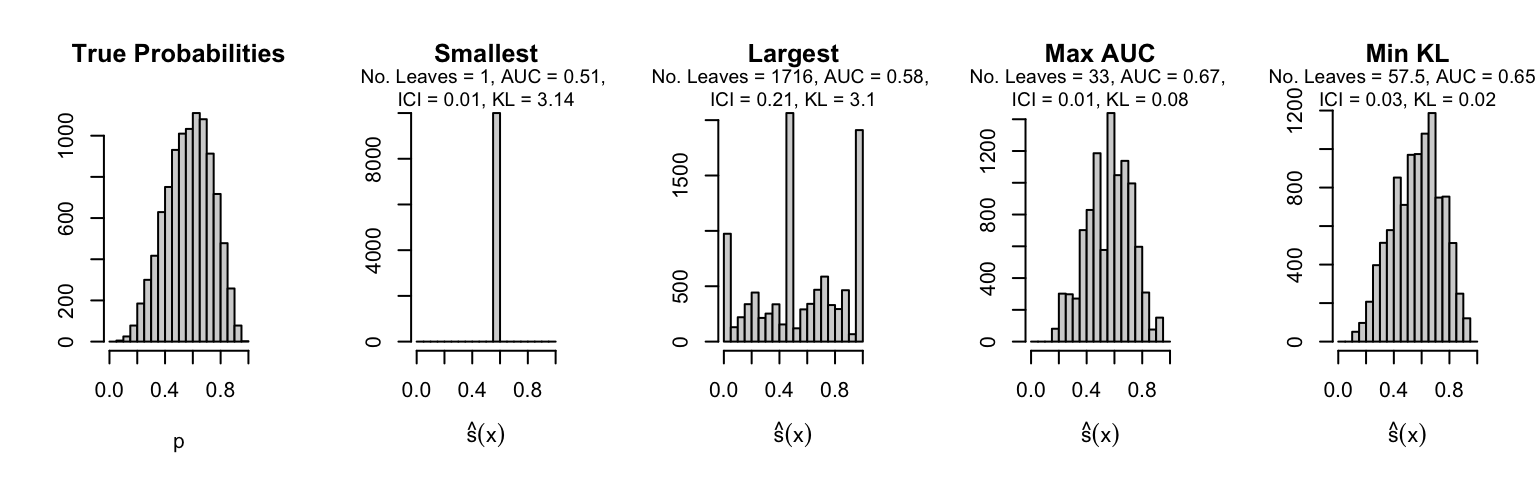
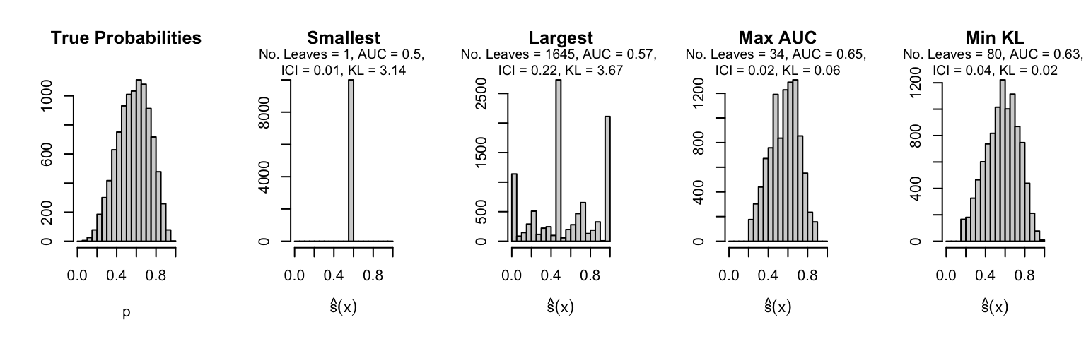
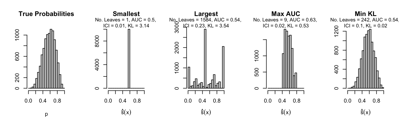
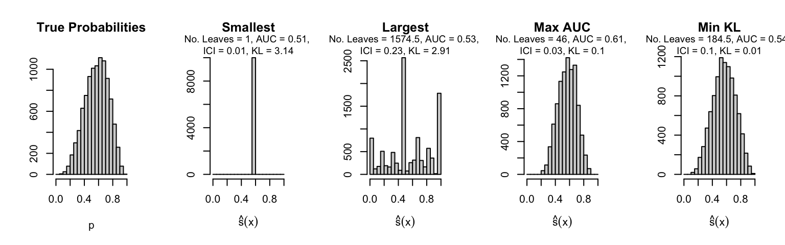
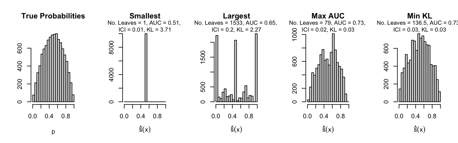
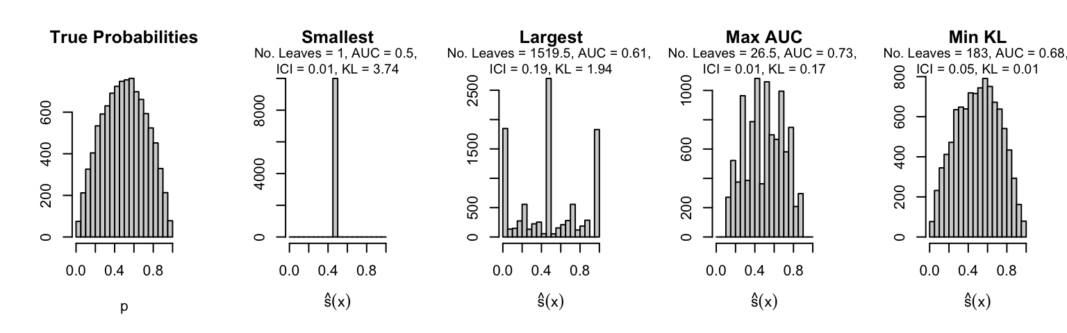
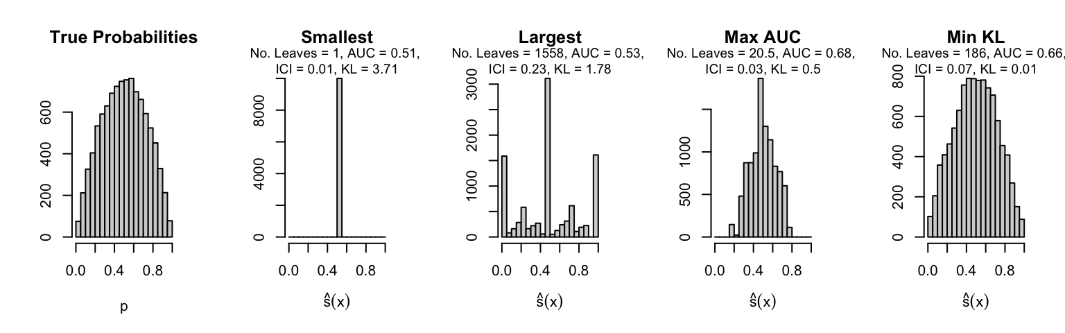
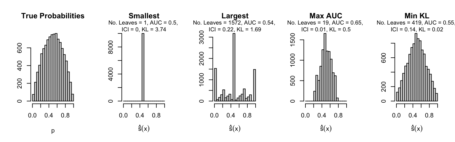
7.5.1.1 Distribution of Scores
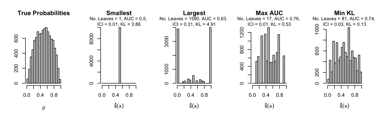
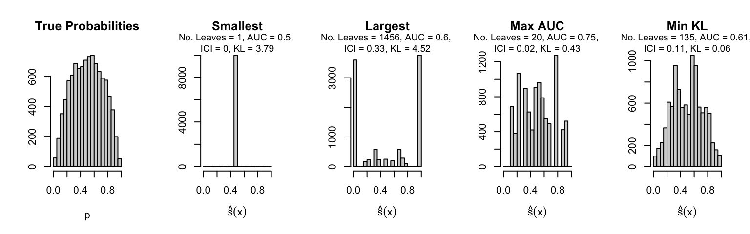
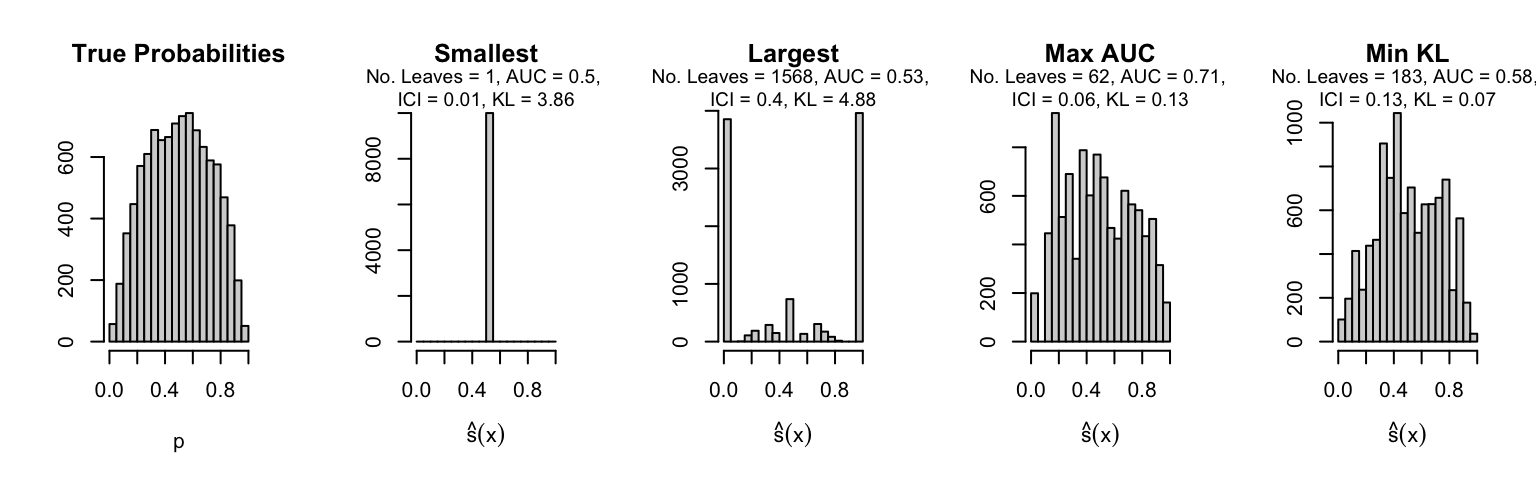
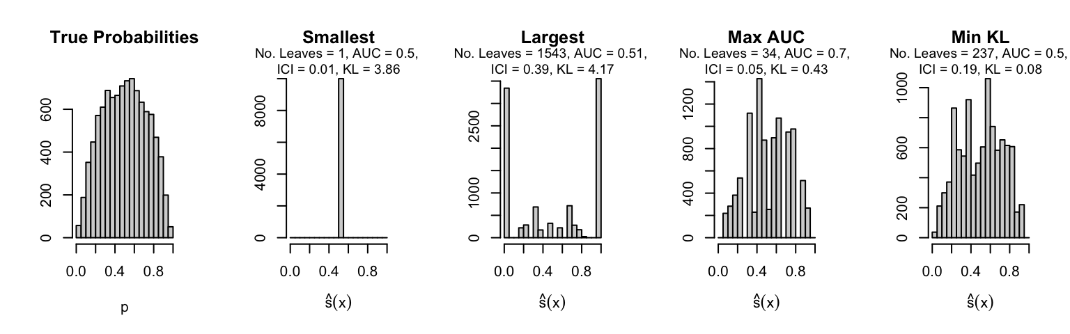
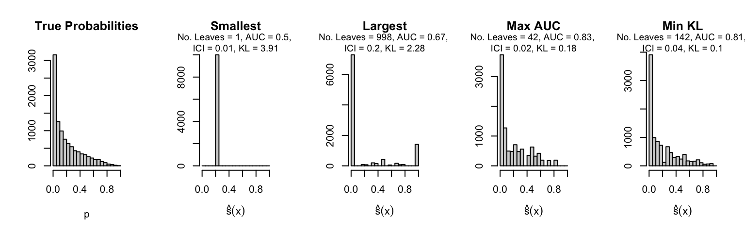
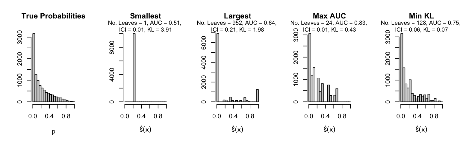
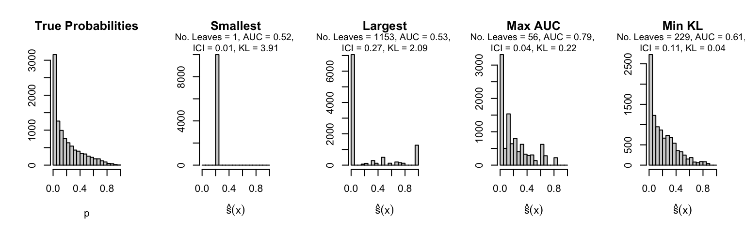
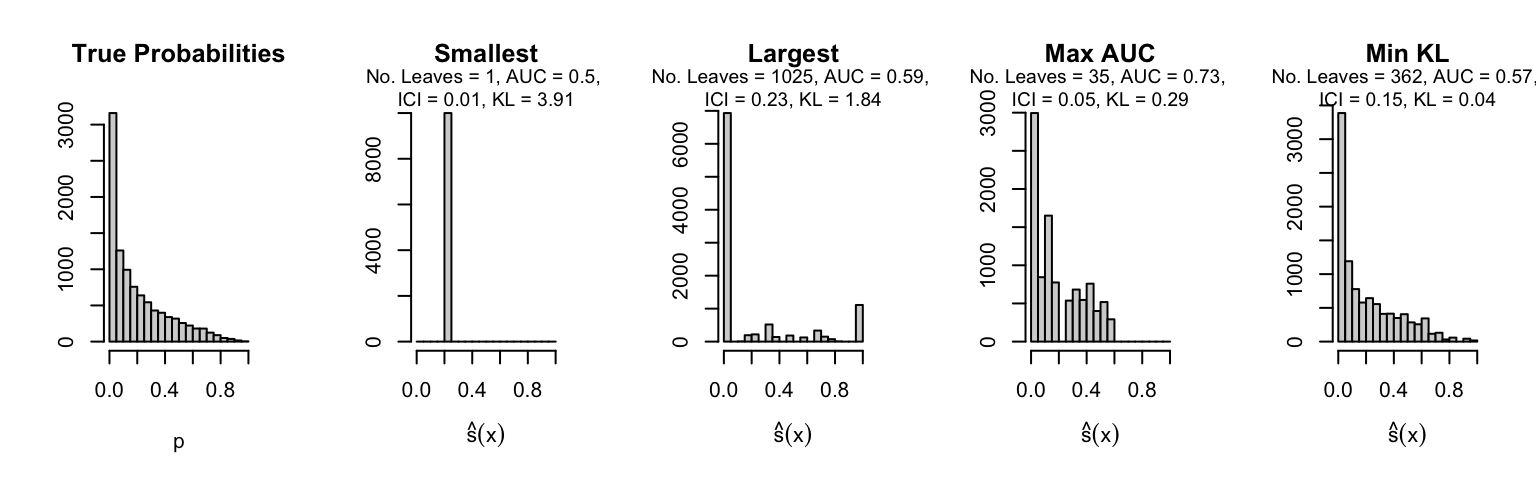
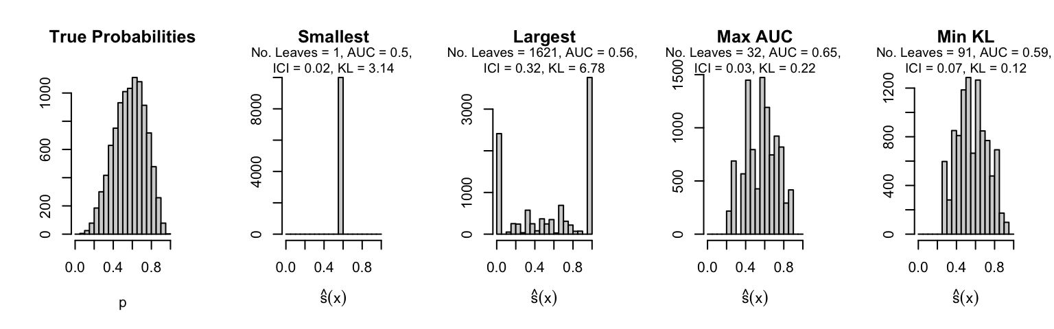
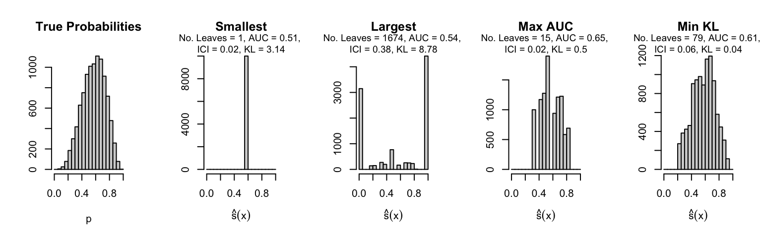
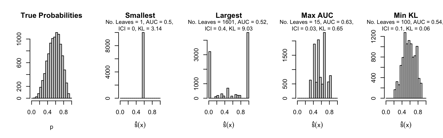
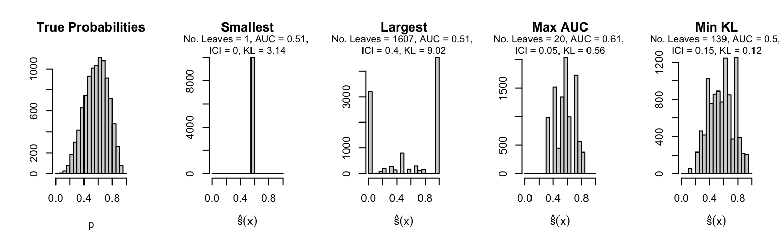
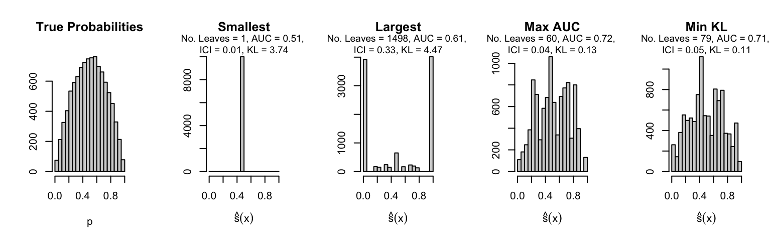
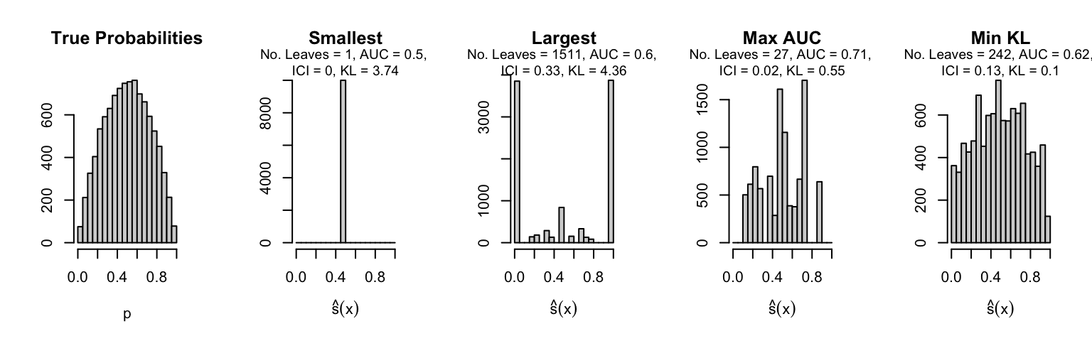
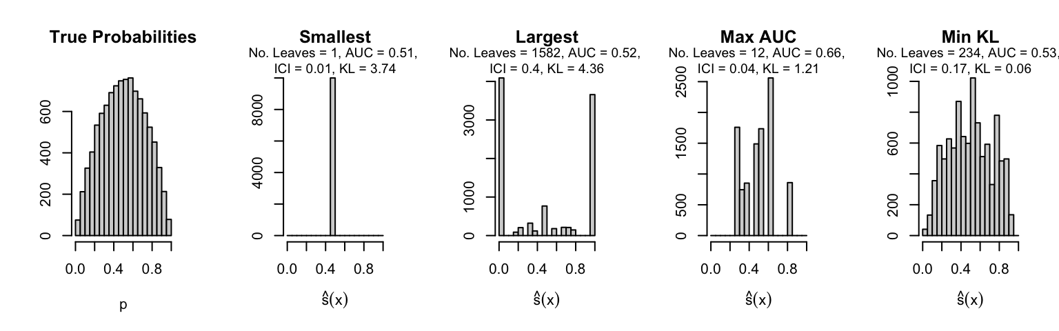
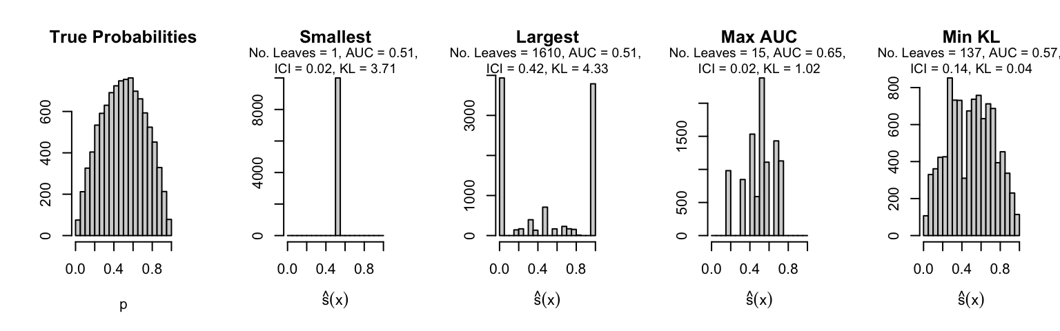
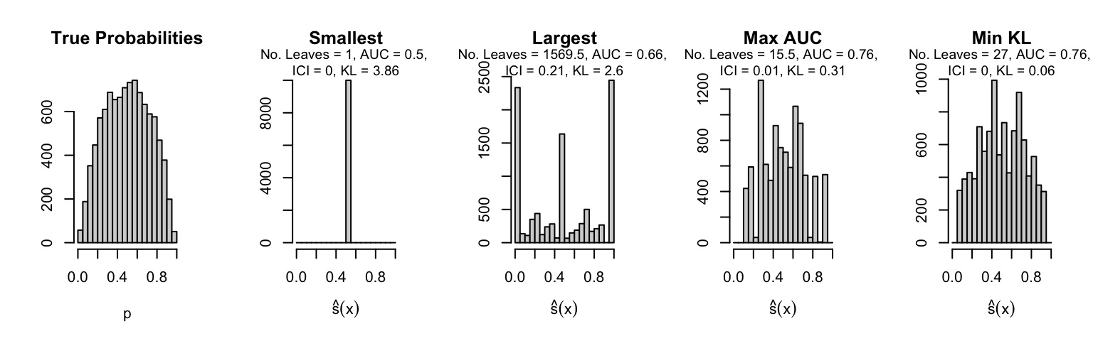
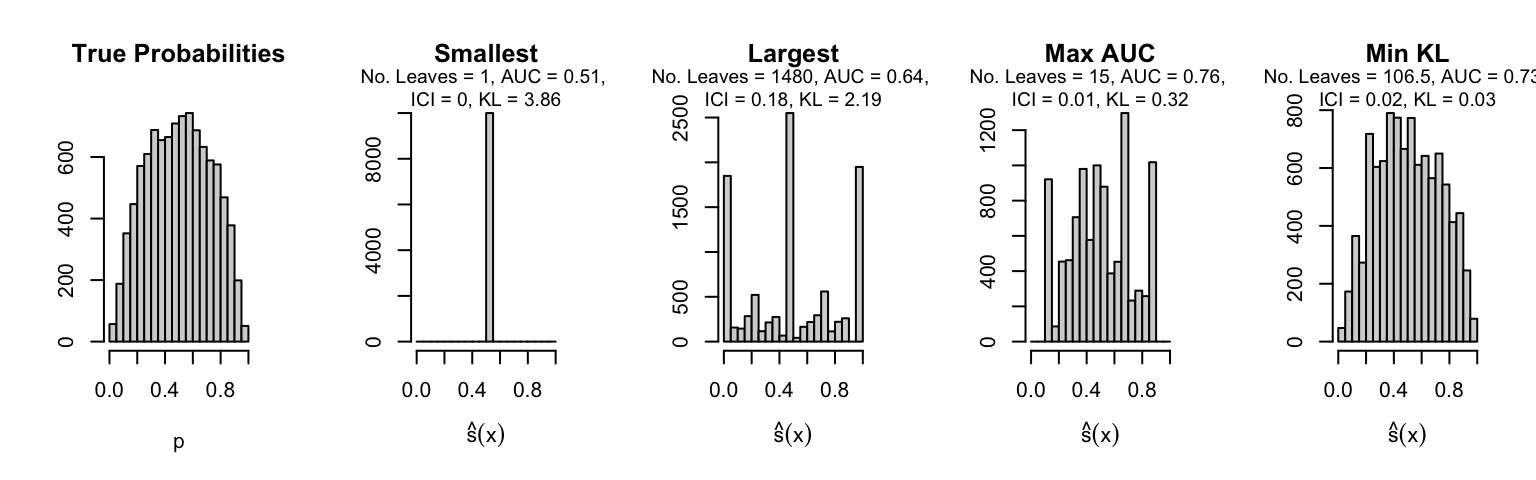
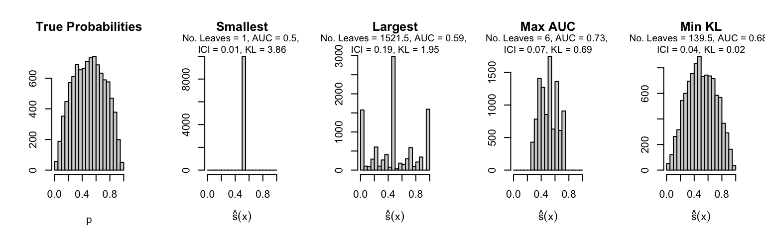
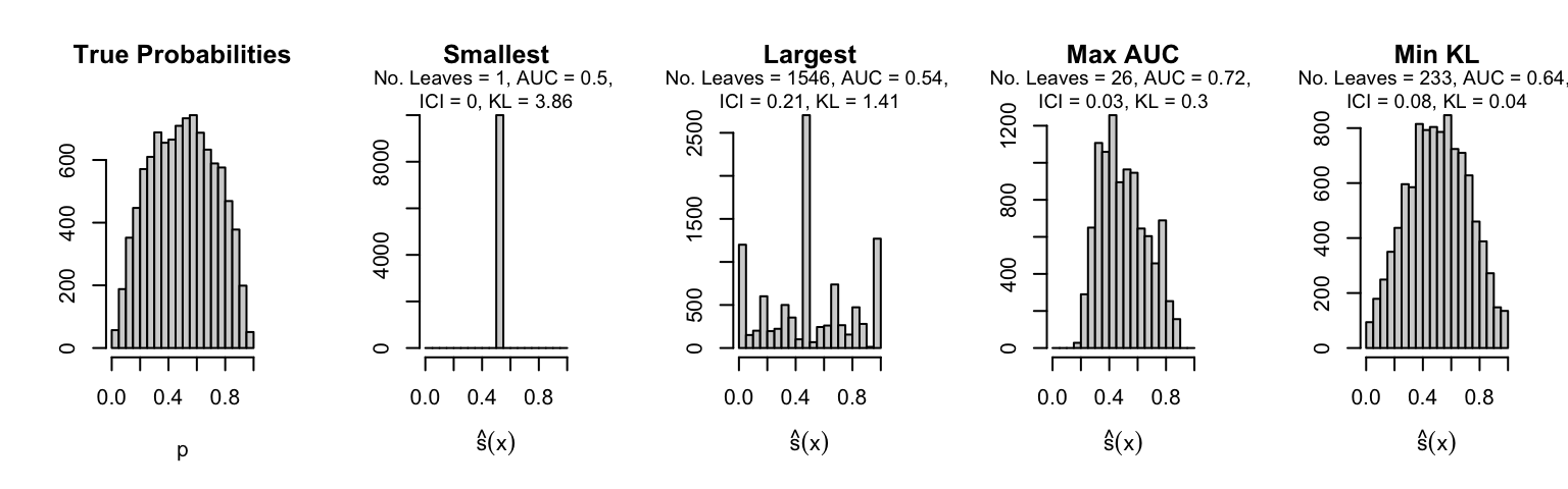
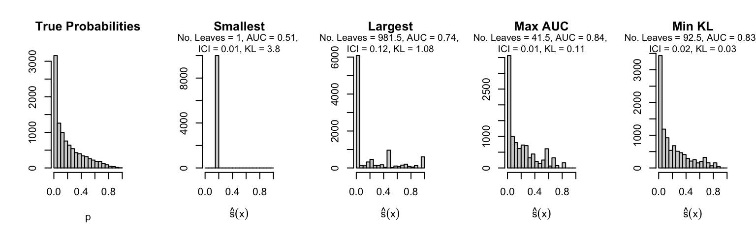
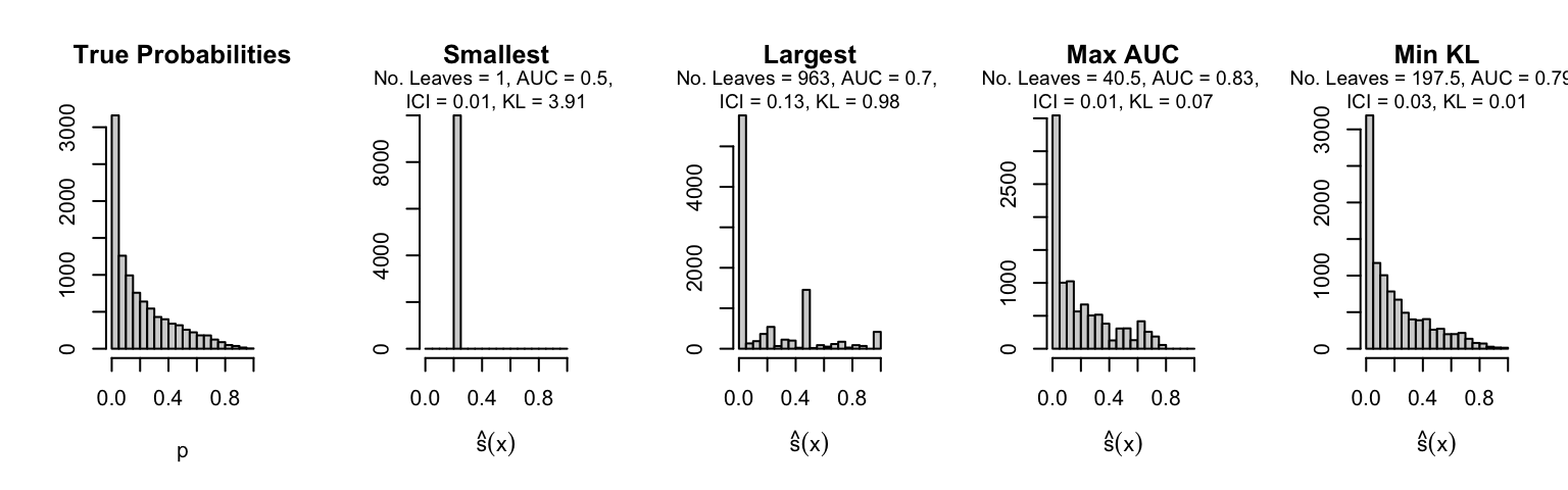
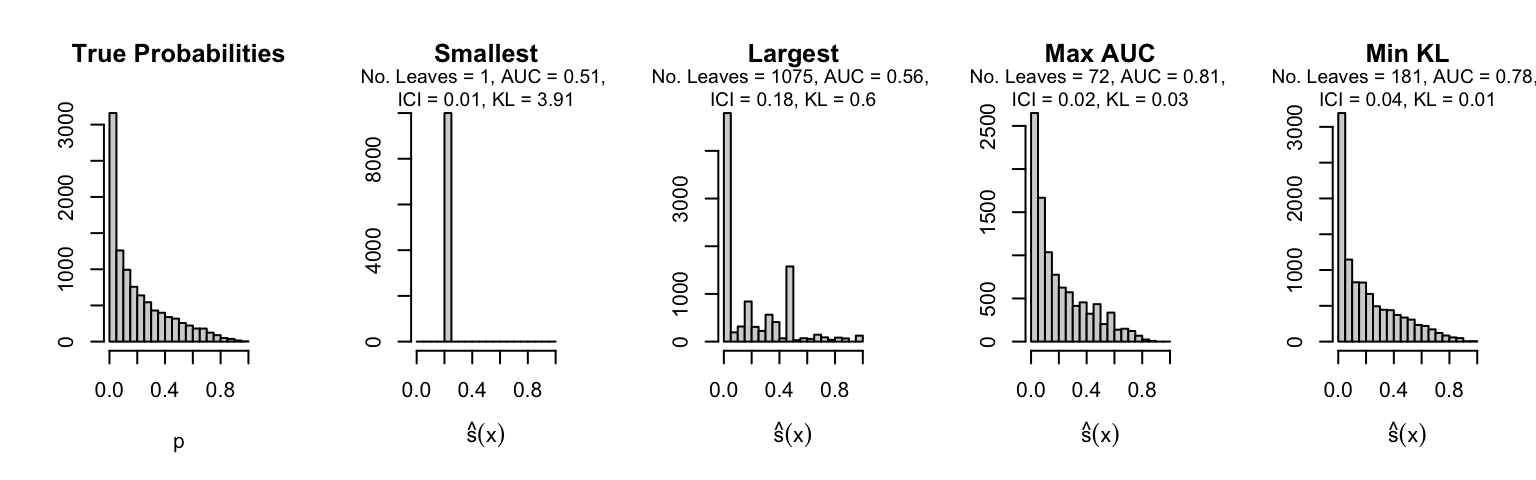
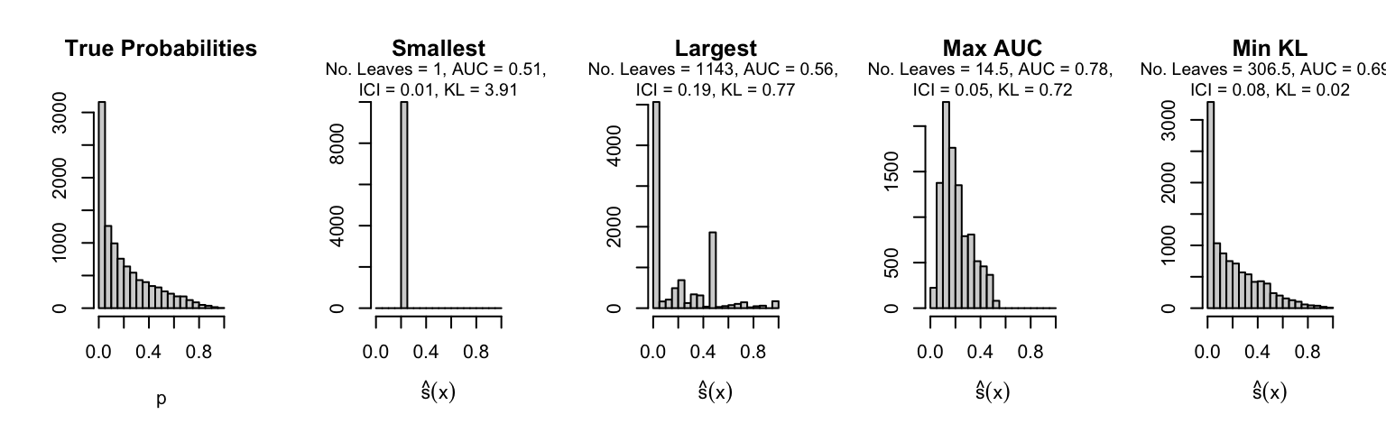
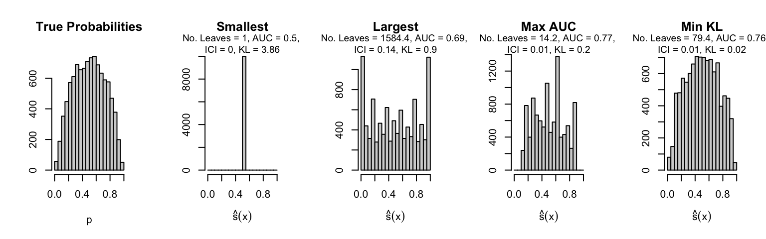
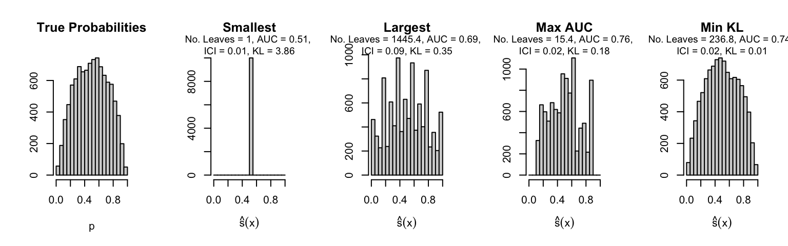
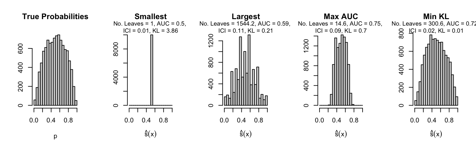
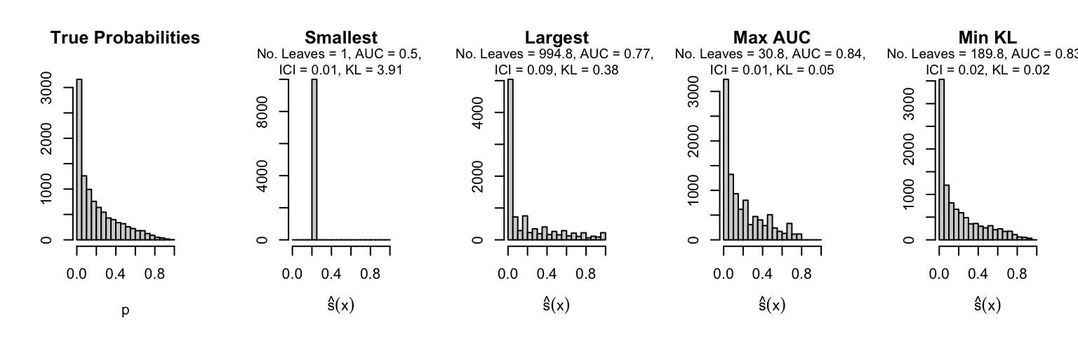
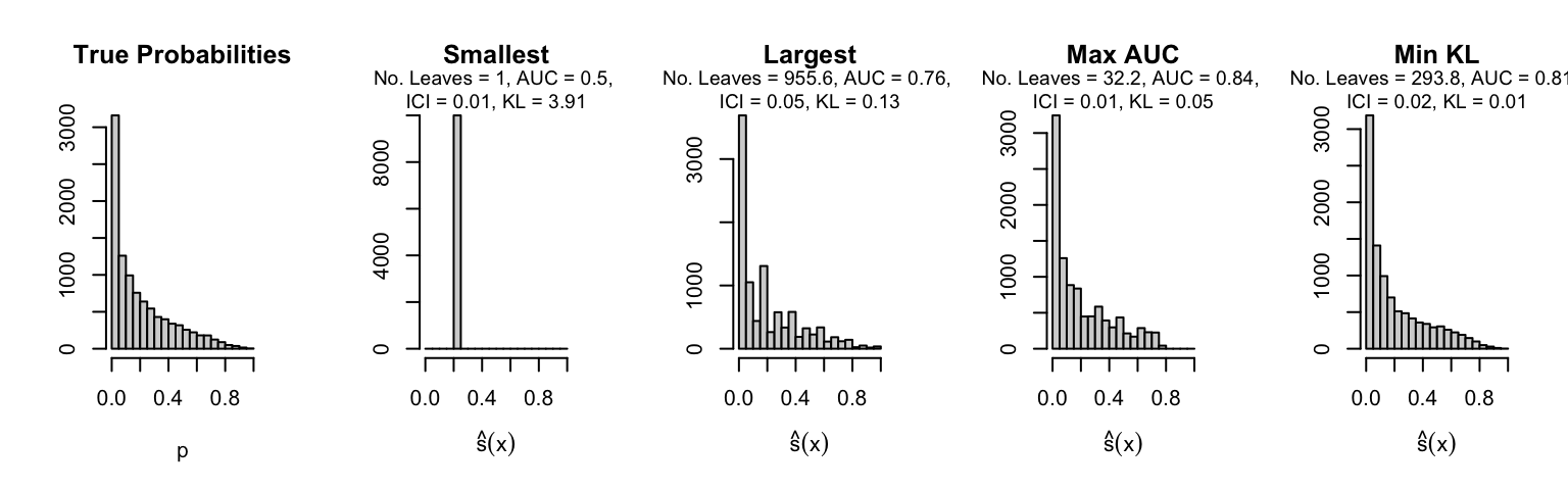
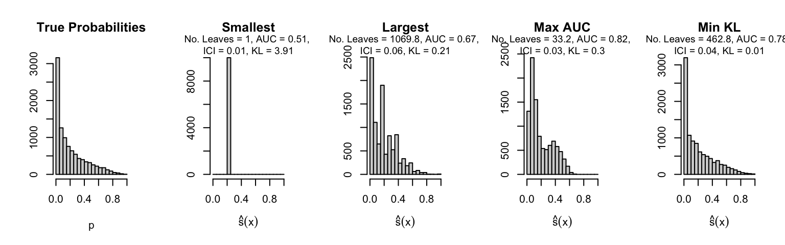
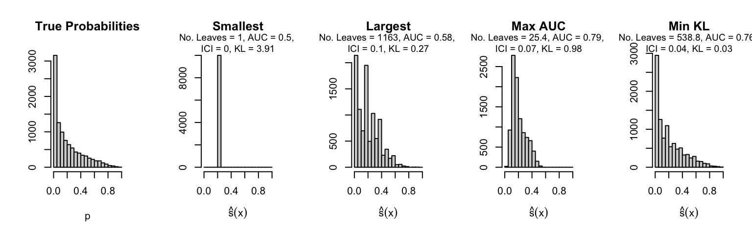
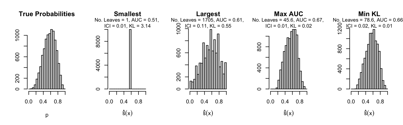
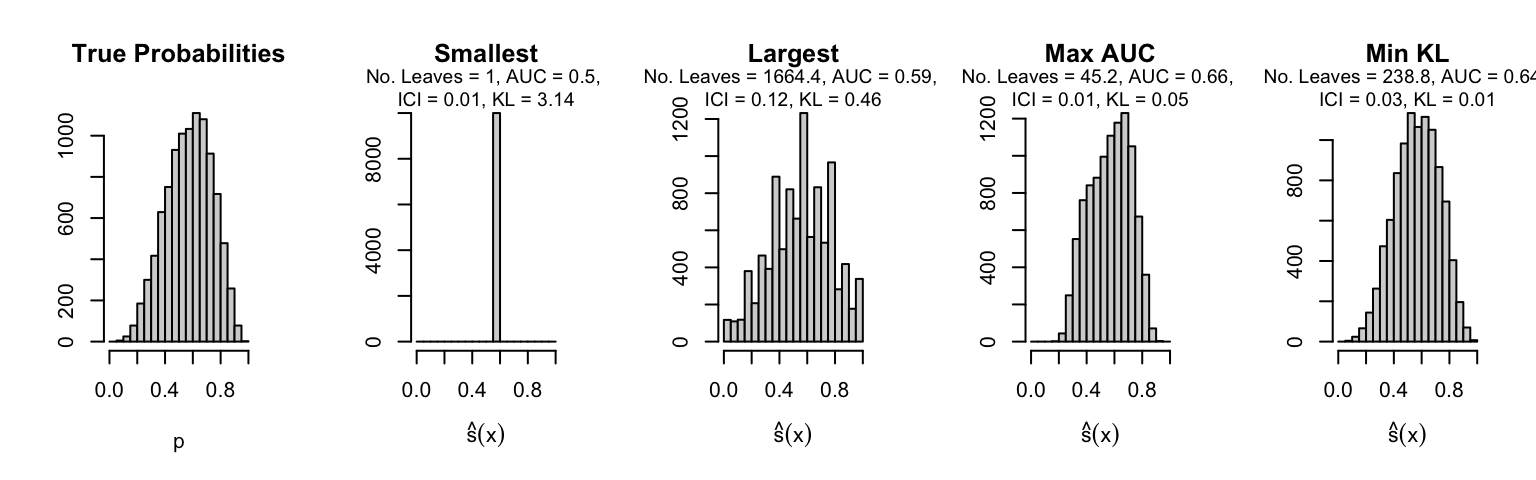
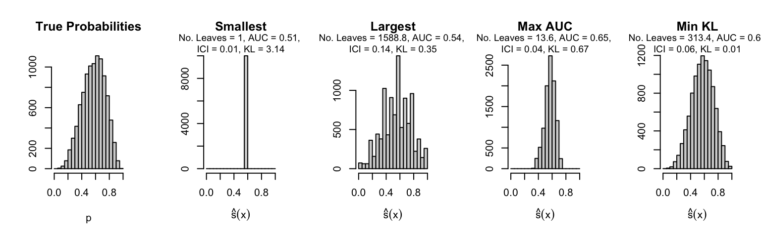
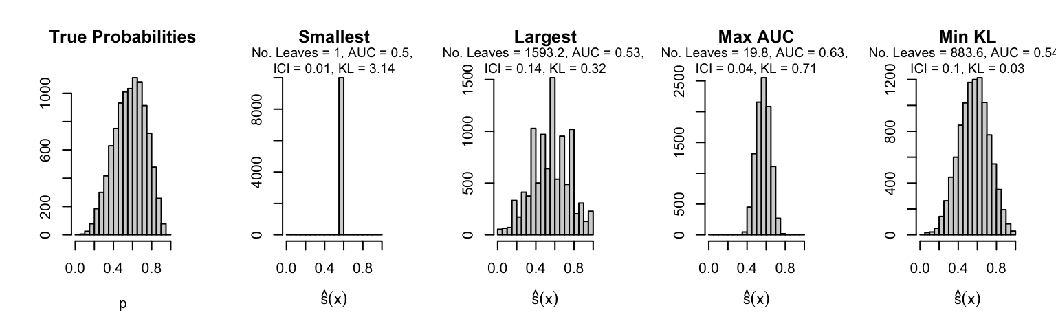
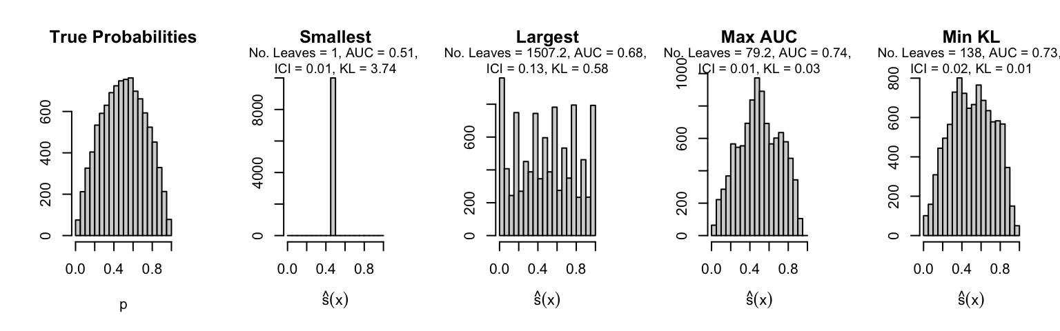
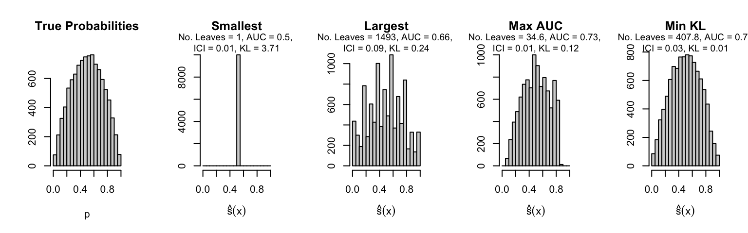
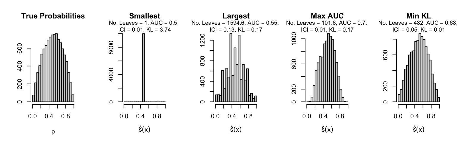
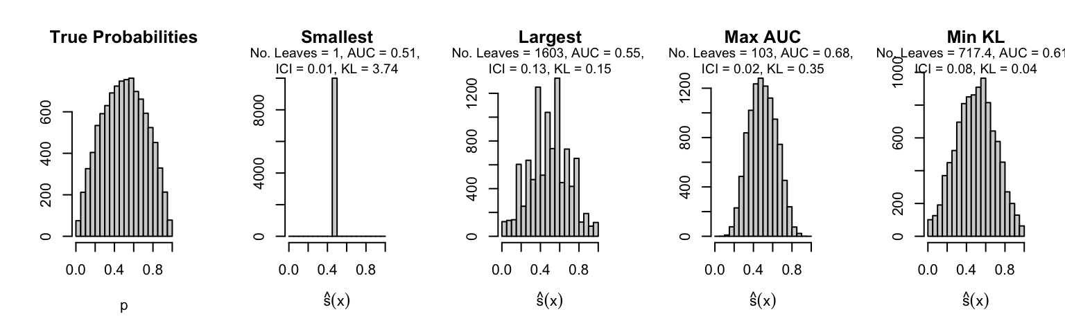
Let us plot the distributions of scores for the trees of interest (smallest, largest, max AUC, min MSE, min KL) for a single replication (the first replication) for each scenario.
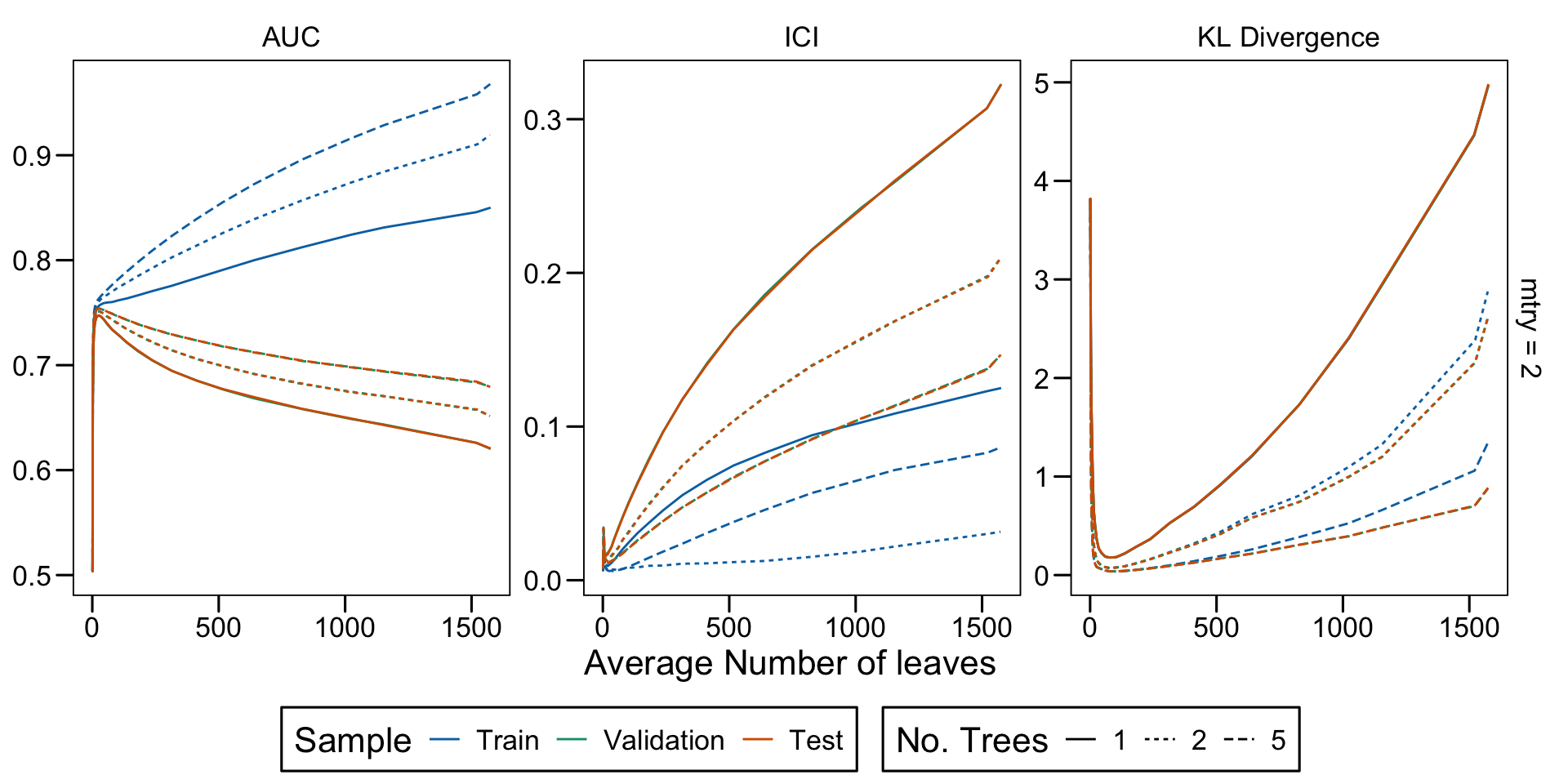
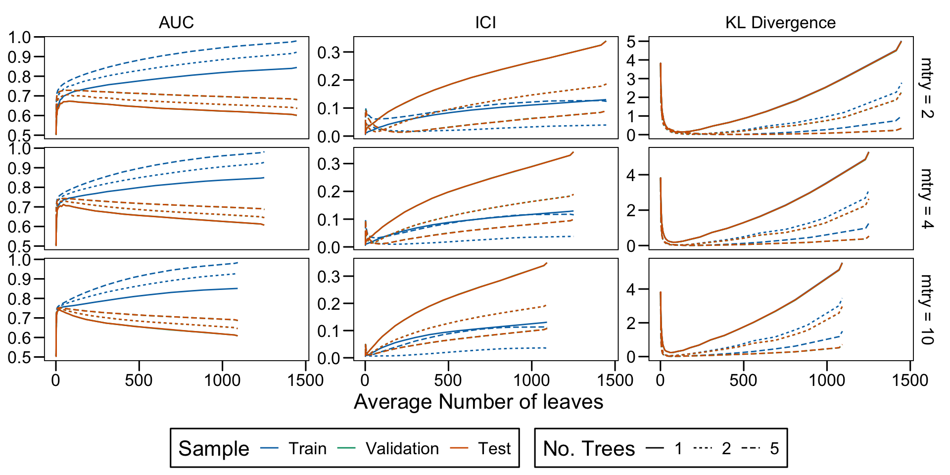
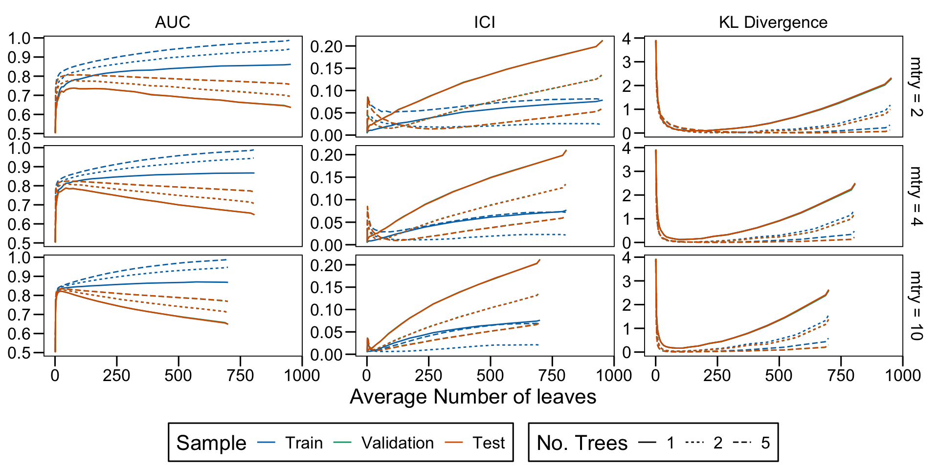
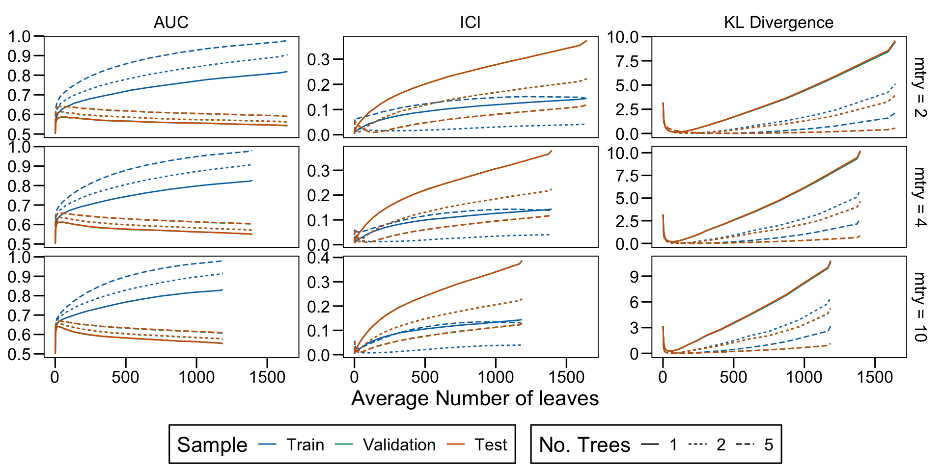
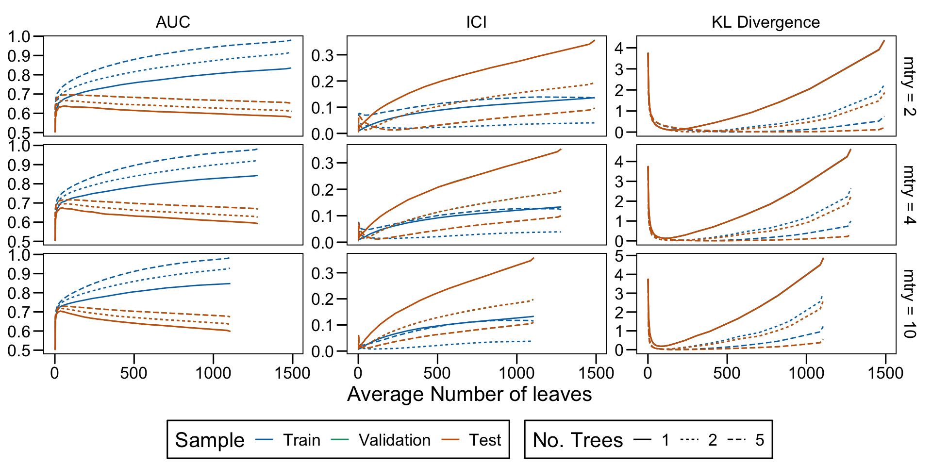
Metrics as a function of the average number of leaves in the trees of the trained forests (DGP 4, 0 noise variables)
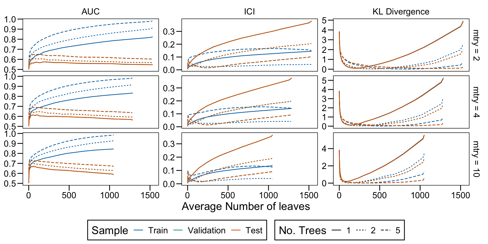
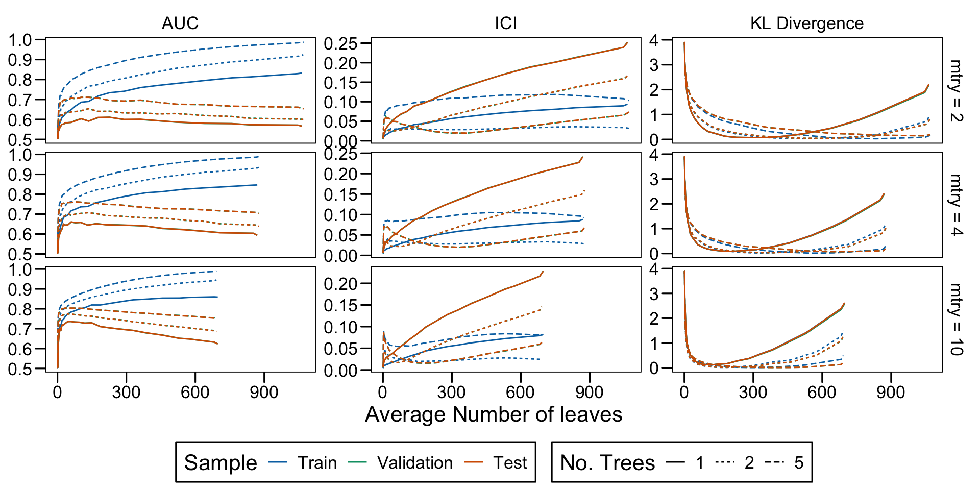
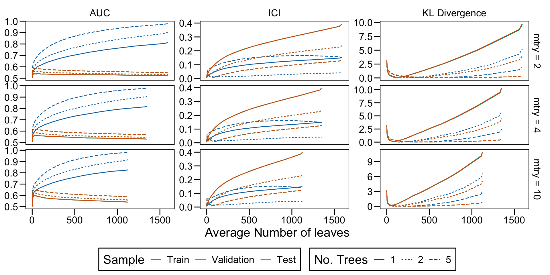
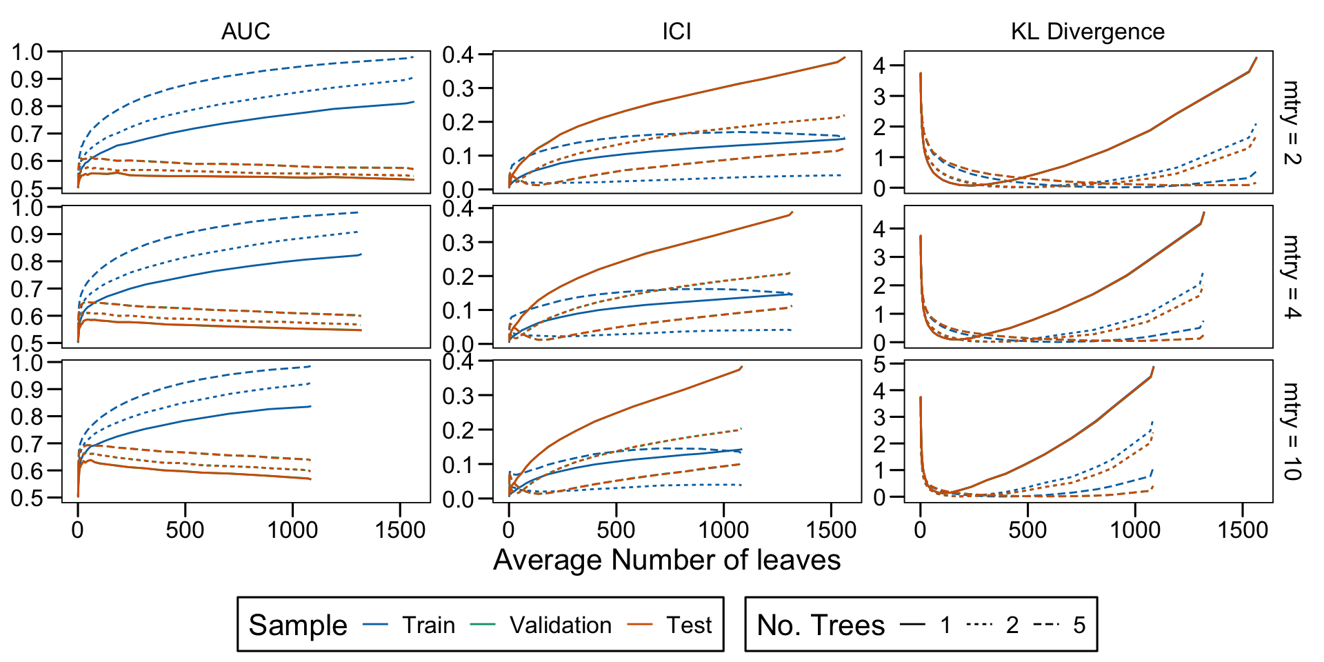
Metrics as a function of the average number of leaves in the trees of the trained forests (DGP 4, 10 noise variables)
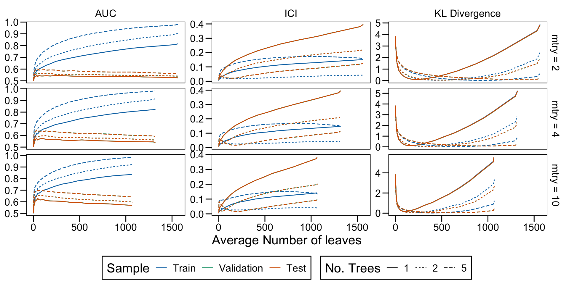
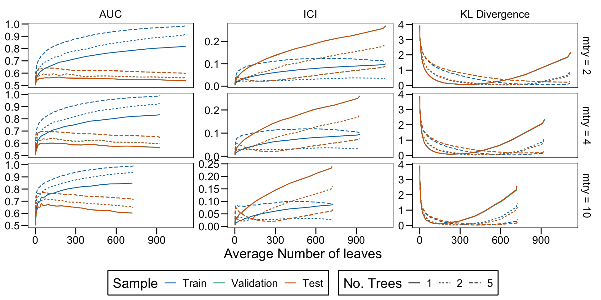
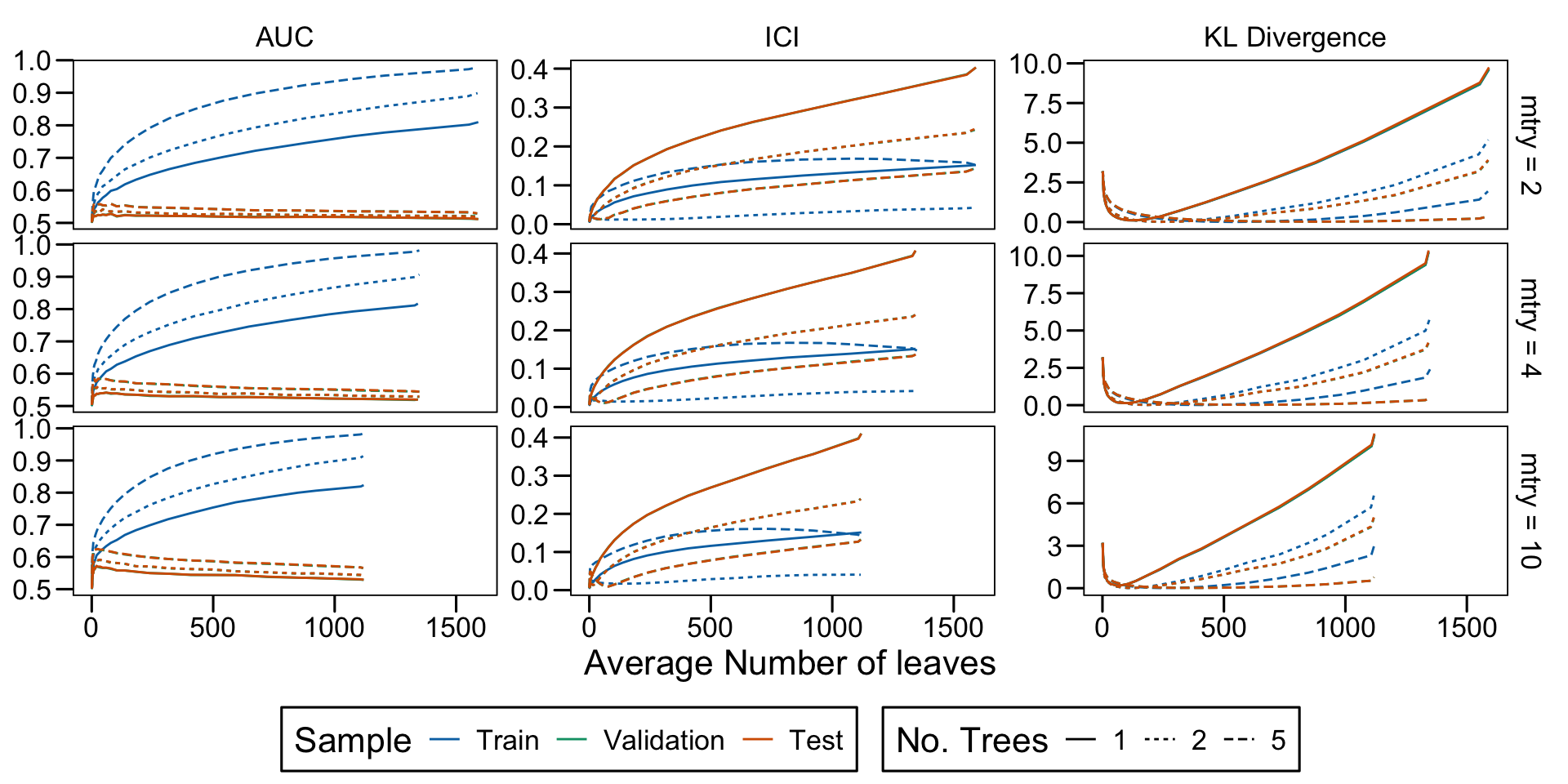
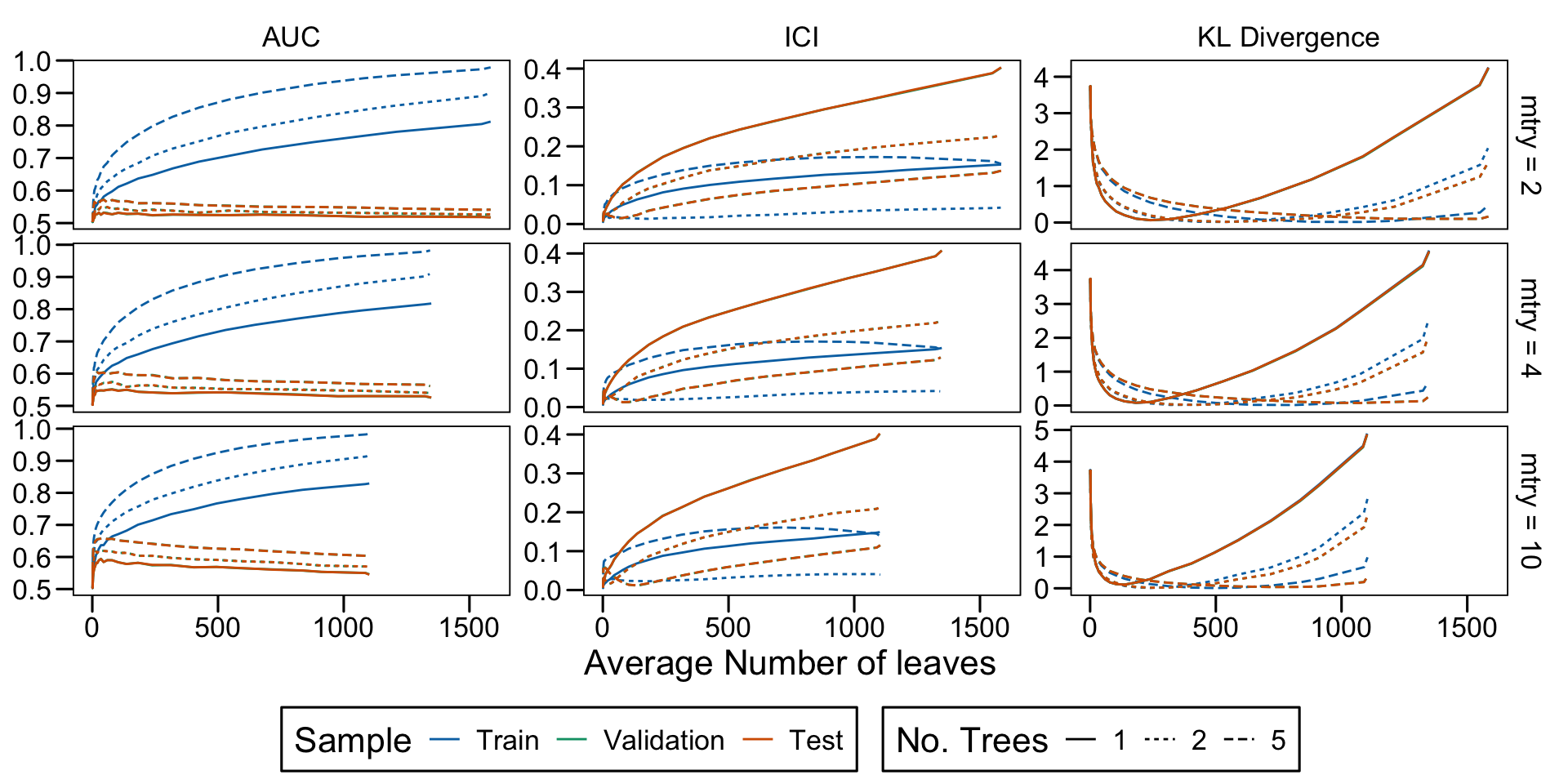
Metrics as a function of the average number of leaves in the trees of the trained forests (DGP 4, 50 noise variables)
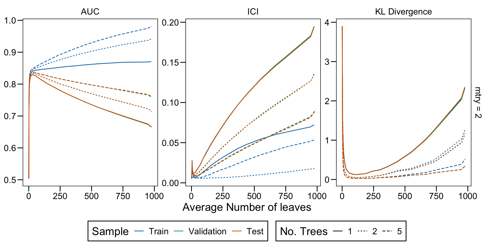
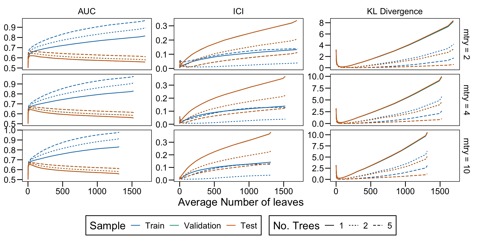
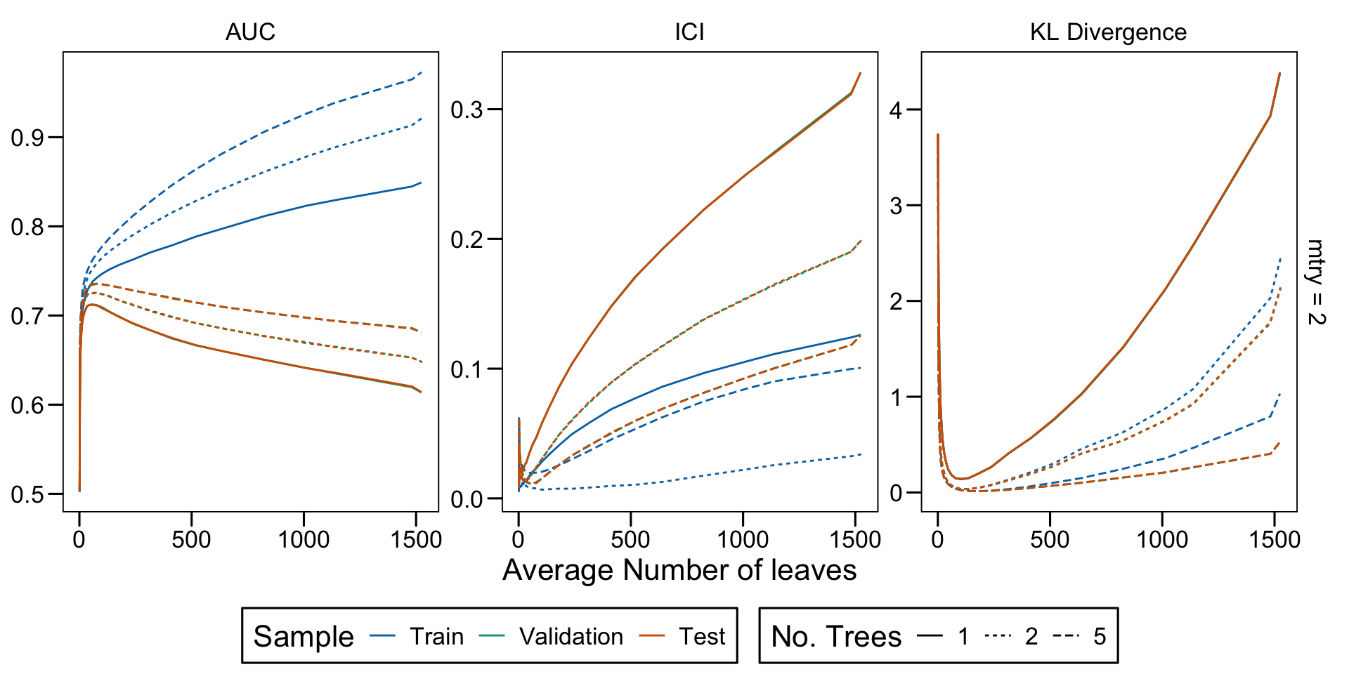
Metrics as a function of the average number of leaves in the trees of the trained forests (DGP 4, 100 noise variables)
Ojeda, Francisco M., Max L. Jansen, Alexandre Thiéry, Stefan Blankenberg, Christian Weimar, Matthias Schmid, and Andreas Ziegler. 2023. “Calibrating Machine Learning Approaches for Probability Estimation: A Comprehensive Comparison.”Statistics in Medicine 42 (29): 5451–78. https://doi.org/10.1002/sim.9921.