11  Generalized Additive Model Selection

Note

This chapter examines the scores returned by a GAMSEL (Generalized Additive Model Selection, Chouldechova and Hastie (2015)) under the different scenarios.

library(tidyverse)

── Attaching core tidyverse packages ──────────────────────── tidyverse 2.0.0 ──
✔ dplyr     1.1.4     ✔ readr     2.1.5
✔ forcats   1.0.0     ✔ stringr   1.5.1
✔ ggplot2   3.5.1     ✔ tibble    3.2.1
✔ lubridate 1.9.3     ✔ tidyr     1.3.1
✔ purrr     1.0.2     
── Conflicts ────────────────────────────────────────── tidyverse_conflicts() ──
✖ dplyr::filter() masks stats::filter()
✖ dplyr::lag()    masks stats::lag()
ℹ Use the conflicted package (<http://conflicted.r-lib.org/>) to force all conflicts to become errors

library(gamsel)

Loaded gamsel 1.8-4

library(philentropy)
library(caret) # for one hot encoding

Loading required package: lattice

Attaching package: 'caret'

The following object is masked from 'package:purrr':

    lift

# Colours for train/test
colour_samples <- c(
  "Train" = "#0072B2",
  "Test" = "#D55E00"
)

#' Theme for ggplot2
#'
#' @param ... arguments passed to the theme function
#' @export
#' @importFrom ggplot2 element_rect element_text element_blank element_line unit
#'   rel
theme_paper <- function (...) {
  ggthemes::theme_base() +
    theme(
      plot.background = element_blank(),
      legend.background = element_rect(
        fill = "transparent", linetype="solid", colour ="black"),
      legend.position = "bottom",
      legend.direction = "horizontal",
      legend.box = "horizontal",
      legend.key = element_blank()
    )
}

11.1 Data

We generate data using the first 12 scenarios from Ojeda et al. (2023) and an additional set of 4 scenarios in which the true probability does not depend on the predictors in a linear way (see Chapter 4).

source("functions/data-ojeda.R")
library(ks)
source("functions/subsample_target_distribution.R")

When we simulate a dataset, we draw the following number of observations:

nb_obs <- 10000

# Coefficients beta
coefficients <- list(
  # First category (baseline, 2 covariates)
  c(0.5, 1),  # scenario 1, 0 noise variable
  c(0.5, 1),  # scenario 2, 10 noise variables
  c(0.5, 1),  # scenario 3, 50 noise variables
  c(0.5, 1),  # scenario 4, 100 noise variables
  # Second category (same as baseline, with lower number of 1s)
  c(0.5, 1),  # scenario 5, 0 noise variable
  c(0.5, 1),  # scenario 6, 10 noise variables
  c(0.5, 1),  # scenario 7, 50 noise variables
  c(0.5, 1),  # scenario 8, 100 noise variables
  # Third category (same as baseline but with 5 num. and 5 categ. covariates)
  c(0.1, 0.2, 0.3, 0.4, 0.5, 0.01, 0.02, 0.03, 0.04, 0.05),
  c(0.1, 0.2, 0.3, 0.4, 0.5, 0.01, 0.02, 0.03, 0.04, 0.05),
  c(0.1, 0.2, 0.3, 0.4, 0.5, 0.01, 0.02, 0.03, 0.04, 0.05),
  c(0.1, 0.2, 0.3, 0.4, 0.5, 0.01, 0.02, 0.03, 0.04, 0.05),
  # Fourth category (nonlinear predictor, 3 covariates)
  c(0.5, 1, .3),  # scenario 5, 0 noise variable
  c(0.5, 1, .3),  # scenario 6, 10 noise variables
  c(0.5, 1, .3),  # scenario 7, 50 noise variables
  c(0.5, 1, .3)  # scenario 8, 100 noise variables
)

# Mean parameter for the normal distribution to draw from to draw num covariates
mean_num <- list(
  # First category (baseline, 2 covariates)
  rep(0, 2),  # scenario 1, 0 noise variable
  rep(0, 2),  # scenario 2, 10 noise variables
  rep(0, 2),  # scenario 3, 50 noise variables
  rep(0, 2),  # scenario 4, 100 noise variables
  # Second category (same as baseline, with lower number of 1s)
  rep(0, 2),  # scenario 5, 0 noise variable
  rep(0, 2),  # scenario 6, 10 noise variables
  rep(0, 2),  # scenario 7, 50 noise variables
  rep(0, 2),  # scenario 8, 100 noise variables
  # Third category (same as baseline but with 5 num. and 5 categ. covariates)
  rep(0, 5),
  rep(0, 5),
  rep(0, 5),
  rep(0, 5),
  # Fourth category (nonlinear predictor, 3 covariates)
  rep(0, 3),
  rep(0, 3),
  rep(0, 3),
  rep(0, 3)
)
# Sd parameter for the normal distribution to draw from to draw num covariates
sd_num <- list(
  # First category (baseline, 2 covariates)
  rep(1, 2),  # scenario 1, 0 noise variable
  rep(1, 2),  # scenario 2, 10 noise variables
  rep(1, 2),  # scenario 3, 50 noise variables
  rep(1, 2),  # scenario 4, 100 noise variables
  # Second category (same as baseline, with lower number of 1s)
  rep(1, 2),  # scenario 5, 0 noise variable
  rep(1, 2),  # scenario 6, 10 noise variables
  rep(1, 2),  # scenario 7, 50 noise variables
  rep(1, 2),  # scenario 8, 100 noise variables
  # Third category (same as baseline but with 5 num. and 5 categ. covariates)
  rep(1, 5),
  rep(1, 5),
  rep(1, 5),
  rep(1, 5),
  # Fourth category (nonlinear predictor, 3 covariates)
  rep(1, 3),
  rep(1, 3),
  rep(1, 3),
  rep(1, 3)
)

params_df <- tibble(
  scenario = 1:16,
  coefficients = coefficients,
  n_num = c(rep(2, 8), rep(5, 4), rep(3, 4)),
  add_categ = c(rep(FALSE, 8), rep(TRUE, 4), rep(FALSE, 4)),
  n_noise = rep(c(0, 10, 50, 100), 4),
  mean_num = mean_num,
  sd_num = sd_num,
  size_train = rep(nb_obs, 16),
  size_test = rep(nb_obs, 16),
  transform_probs = c(rep(FALSE, 4), rep(TRUE, 4), rep(FALSE, 4), rep(FALSE, 4)),
  linear_predictor = c(rep(TRUE, 12), rep(FALSE, 4)),
  seed = 202105
)
rm(coefficients, mean_num, sd_num)

11.2 Metrics

We load the functions from Chapter 3 to compute performance, calibration and divergence metrics.

source("functions/metrics.R")

11.3 Simulations Setup

As in previous chapters, we define a function to run replications of the simulations for each scenario. This function is called simul_gamsel(). It uses multiple helper functions also defined here.

#' Counts the number of scores in each of the 20 equal-sized bins over [0,1]
#'
#' @param scores_train vector of scores on the train test
#' @param scores_test vector of scores on the test test
get_histogram <- function(scores_train, scores_test) {
  breaks <- seq(0, 1, by = .05)
  scores_train_hist <- hist(scores_train, breaks = breaks, plot = FALSE)
  scores_test_hist <- hist(scores_test, breaks = breaks, plot = FALSE)
  scores_hist <- list(
    train = scores_train_hist,
    test = scores_test_hist
  )
  scores_hist
}

#' Get KL divergence metrics for estimated scores and true probabilities
#' 
#' @param scores_train vector of scores on the train test
#' @param scores_test vector of scores on the test test
#' @param true_prob list of true probabilities on train and test set
get_disp_metrics <- function(scores_train, scores_test, true_prob) {
  disp_train <- dispersion_metrics(
    true_probas = true_prob$train, scores = scores_train
  ) |> mutate(sample = "train")
  disp_test <- dispersion_metrics(
    true_probas = true_prob$test, scores = scores_test
  ) |> mutate(sample = "test")
  
  tb_disp_metrics <- disp_train |>
    bind_rows(disp_test)
  tb_disp_metrics
}

#' Get the performance and calibration metrics for estimated scores
#' 
#' @param scores_train vector of scores on the train test
#' @param scores_test vector of scores on the test test
#' @param tb_train train set
#' @param tb_test test set
#' @param true_prob list of true probabilities on train and test set
get_perf_metrics <- function(scores_train, 
                             scores_test,
                             tb_train,
                             tb_test,
                             true_prob) {
  # We add very small noise to predicted scores
  # otherwise the local regression may crash
  scores_train_noise <- scores_train +
    runif(n = length(scores_train), min = 0, max = 0.01)
  scores_train_noise[scores_train_noise > 1] <- 1
  metrics_train <- compute_metrics(
    obs = tb_train$d, scores = scores_train_noise, true_probas = true_prob$train
  ) |> mutate(sample = "train")
  
  scores_test_noise <- scores_test +
    runif(n = length(scores_test), min = 0, max = 0.01)
  scores_test_noise[scores_test_noise > 1] <- 1
  metrics_test <- compute_metrics(
    obs = tb_test$d, scores = scores_test_noise, true_probas = true_prob$test
  ) |> mutate(sample = "test")
  
  tb_metrics <- metrics_train |>
    bind_rows(metrics_test)
  tb_metrics
}

#' Estimation of P(q1 < score < q2)
#' 
#' @param scores_train vector of scores on the train test
#' @param scores_test vector of scores on the test test
#' @param q1 vector of desired values for q1 (q2 = 1-q1)
estim_prop <- function(scores_train, 
                       scores_test, 
                       q1 = c(.1, .2, .3, .4)) {
  proq_scores_train <- map(
    q1,
    ~prop_btw_quantiles(s = scores_train, q1 = .x)
  ) |>
    list_rbind() |>
    mutate(sample = "train")
  proq_scores_test <- map(
    q1,
    ~prop_btw_quantiles(s = scores_test, q1 = .x)
  ) |>
    list_rbind() |>
    mutate(sample = "test")
  
  proq_scores_train |> 
    bind_rows(proq_scores_test)
}

#' Run a single replication of the simulations of a scenario
#' Fits a GAMSEL model to the data.
#' 
#' @param scenario ID of the scenario
#' @param params_df tibble with the parameters used to generate data
#' @param repn replication ID number
simul_gamsel <- function(scenario, params_df, repn) {
  # Generate Data----
  simu_data <- simulate_data_wrapper(
    scenario = scenario,
    params_df = params_df,
    repn = repn
  )

  tb_train <- simu_data$data$train |> rename(d = y)
  tb_test <- simu_data$data$test |> rename(d = y)

  true_prob <-
    list(
      train = simu_data$data$probs_train,
      test = simu_data$data$probs_test
    )

  # Format Data----

  if (scenario %in% 9:12) {
    # Factor variables
    tb_train <- tb_train |> mutate(across(x6:x10, as.factor))
    tb_test <- tb_test |> mutate(across(x6:x10, as.factor))
  }

  X_train <- tb_train |> select(-d)
  X_test <- tb_test |> select(-d)
  y_train <- tb_train |> pull(d)
  ## One hot encoding
  dmy_train <- dummyVars(
    " ~ -1+.", data = X_train, fullRank = TRUE, contrasts = TRUE, sep = "."
  )
  X_dmy_train <- data.frame(predict(dmy_train, newdata = X_train))
  # using same encoder for test set
  X_dmy_test <- data.frame(predict(dmy_train, newdata = X_test))
  categ_names <- map2(
    .x = dmy_train$facVars, .y = dmy_train$lvls, .f = ~str_c(.x, ".", .y)
  ) |>
    unlist()

  # Estimation----
  ## Degrees
  deg <- ifelse(!colnames(X_dmy_train) %in% categ_names, 5, 1)
  gamsel_cv <- cv.gamsel(
    x = X_dmy_train, y = y_train, family="binomial", degrees = deg
  )
  gamsel_out <- gamsel(
    x = X_dmy_train, y = y_train, family = "binomial", degrees = deg,
    lambda = gamsel_cv$lambda.min
  )

  # Predicted scores----
  scores_train <- predict(
    gamsel_out, newdata = X_dmy_train, type = "response")[, 1]
  scores_test <- predict(
    gamsel_out, newdata = X_dmy_test, type = "response")[, 1]

  # Histogram of scores----
  scores_hist <- get_histogram(scores_train, scores_test)

  # Performance and Calibration Metrics----
  tb_metrics <- get_perf_metrics(
    scores_train = scores_train,
    scores_test = scores_test,
    tb_train = tb_train,
    tb_test = tb_test,
    true_prob = true_prob) |>
    mutate(
      scenario = simu_data$scenario,
      repn = simu_data$repn
    )

  # Dispersion Metrics----
  tb_disp_metrics <- get_disp_metrics(
    scores_train = scores_train,
    scores_test = scores_test,
    true_prob = true_prob
  ) |>
    mutate(
      scenario = simu_data$scenario,
      repn = simu_data$repn
    )

  metrics <- suppressMessages(
    left_join(tb_metrics, tb_disp_metrics)
  )

  # Estimation of P(q1 < score < q2)----
  tb_prop_scores <- estim_prop(scores_train, scores_test) |>
    mutate(
      scenario = simu_data$scenario,
      repn = simu_data$repn
    )

  list(
    scenario = simu_data$scenario,   # data scenario
    repn = simu_data$repn,           # data replication ID
    metrics = metrics,            # table with performance/calib/divergence
    tb_prop_scores = tb_prop_scores, # table with P(q1 < score < q2)
    scores_hist = scores_hist       # histogram of scores
  )
}

The desired number of replications for each scenario needs to be set:

repns_vector <- 1:100

11.4 Estimations

We loop over the 16 scenarios and run the 100 replications in parallel.

library(pbapply)
library(parallel)
ncl <- detectCores()-1
(cl <- makeCluster(ncl))

clusterEvalQ(cl, {
  library(tidyverse)
  library(ks)
  library(gamsel)
  library(philentropy)
  library(caret)
}) |>
  invisible()

clusterExport(
  cl, c(
    # Functions
    "brier_score",
    "compute_metrics",
    "dispersion_metrics",
    "prop_btw_quantiles",
    "subset_target",
    "simulate_data",
    "simulate_data_wrapper",
    "simul_gamsel",
    "get_histogram",
    "get_disp_metrics",
    "get_perf_metrics",
    "estim_prop",
    # Objects
    "grid",
    "params_df",
    "repns_vector"
    )
  )

for (i_scenario in 1:16) {
  scenario <- i_scenario
  print(str_c("Scenario ", scenario, "/", nrow(params_df)))
  clusterExport(cl, c("scenario"))
  resul_gamsel_scenario <-
    pblapply(
      1:length(repns_vector), function(i) simul_gamsel(
        scenario = scenario, params_df = params_df, repn = i
      ),
      cl = cl
    )
  save(
    resul_gamsel_scenario,
    file = str_c("output/simul/dgp-ojeda/resul_gamsel_scenario_", scenario, ".rda")
  )
}
stopCluster(cl)

The results can be loaded as follows:

files <- str_c(
  "output/simul/dgp-ojeda/resul_gamsel_scenario_", 1:16, ".rda"
)
resul_gamsel <- map(files[file.exists(files)], ~{load(.x) ; resul_gamsel_scenario})

The resul_gamsel object is of length 16: each element contains the simulations for a scenario. For each scenario, the elements are a list of length max(repns_vector), i.e., the number of replications. Each replication gives, in a list, the following elements:

• scenario: the number of the scenario
• repn: the replication number
• metrics: the metrics (AUC, Calibration, KL Divergence , etc.) for each model from the grid search, for all boosting iterations.
• tb_prop_scores: the estimations of \(\mathbb{P}(q_1 < \hat{s}(\mathbb{x})< q_2)\), for \(q_1 =\{ .1, .2, .3, .4\}\).
• scores_hist: the counts on bins defined on estimated scores (on both train and test sets).

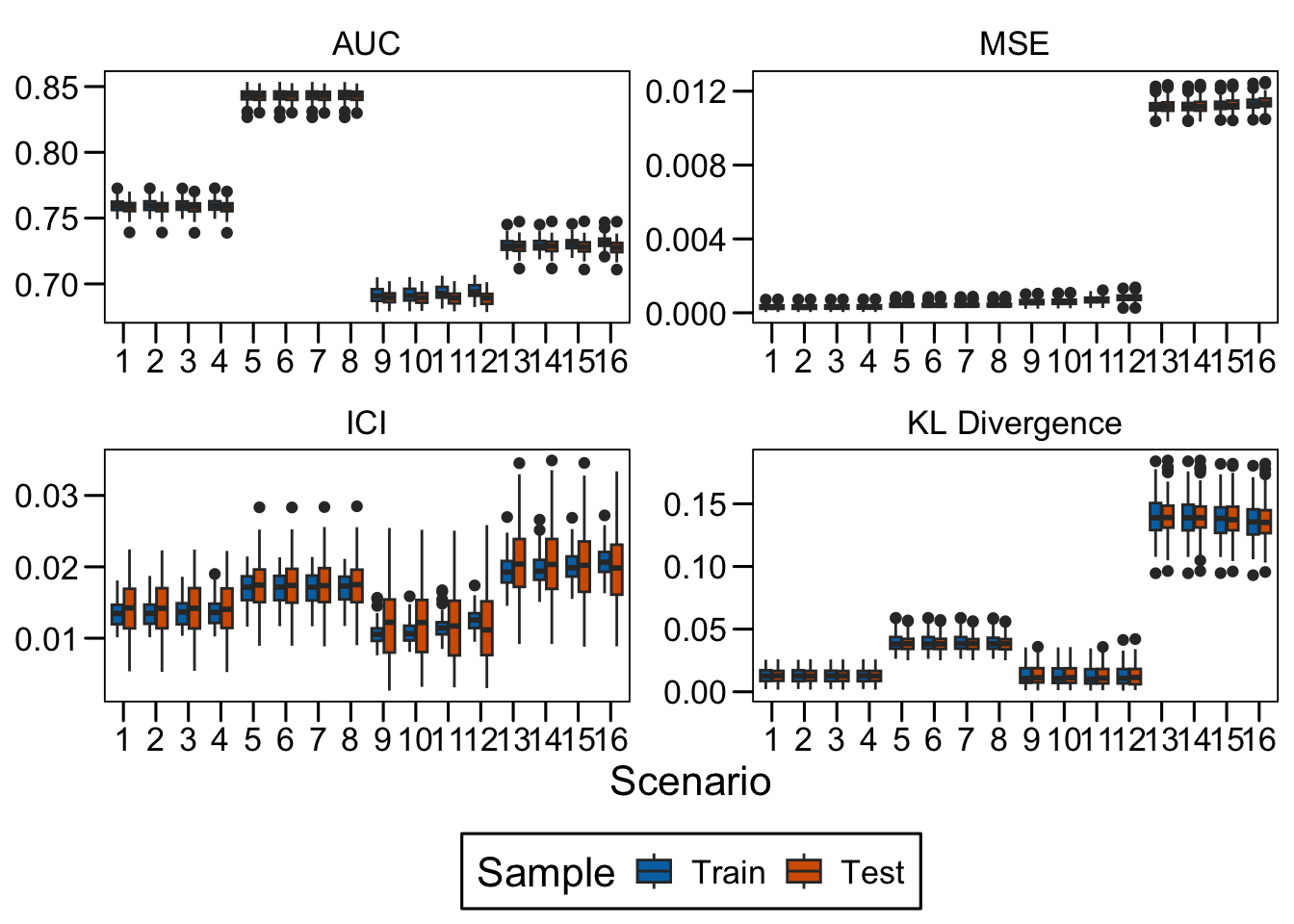
11.5 Results

We can now extract some information from the results. Let us begin with the different metrics computed for each of the replications for each scenario.

metrics_gamsel_all <- map(
  resul_gamsel, 
  function(resul_gamsel_sc) map(resul_gamsel_sc, "metrics") |> list_rbind()
) |> 
  list_rbind()

We can then show boxplots of the metrics for each scenario.

df_plot <- metrics_gamsel_all |> 
  select(scenario, sample, AUC, mse, ici, KL_20_true_probas) |> 
  pivot_longer(cols = -c(scenario, sample), names_to = "metric") |> 
  mutate(
    scenario = factor(scenario),
    sample = factor(
      sample,
      levels = c("train", "test"),
      labels = c("Train", "Test")
    ),
    metric = factor(
      metric,
      levels = c("AUC", "mse", "ici", "KL_20_true_probas"),
      labels = c("AUC", "MSE", "ICI", "KL Divergence")
    )
  )

ggplot(
  data = df_plot,
  mapping = aes(x = scenario, y = value, fill = sample)
) +
  geom_boxplot() +
  facet_wrap(~metric, scales = "free") +
  scale_fill_manual("Sample", values = colour_samples) +
  labs(x = "Scenario", y = NULL) +
  theme_paper()

Figure 11.1: Metrics for the GAMSEL model computed on 100 replications of the simulations for each scenario.

11.5.1 Distribution of Scores

Then, we can have a look at the distribution of scores on the train set and on the test set for each scenario.

scores_hist_all <- 
  map(
    resul_gamsel,
    function(resul_gamsel_sc) map(resul_gamsel_sc, "scores_hist")
  )

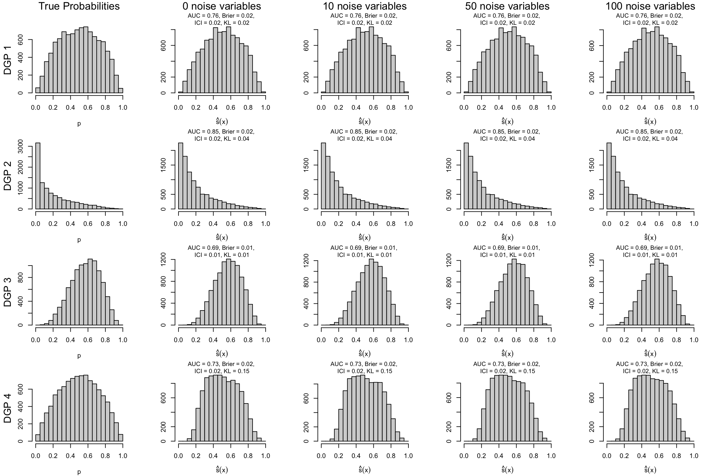
We can focus on the first replication of each of the scenarios:

repn <- 1

We define a function, plot_hist() to plot the distribution of scores also showing some metrics (AUC, ICI and KL divergence) for a particular replication of one scenario. We also define a second function, plot_hist_dgp() to plot the distributions of true probabilities and that of a replication, for multiple scenarios within a DGP.

plot_hist <- function(metrics_interest, scores_hist_interest) {
  subtitle <- str_c(
    "AUC = ", round(metrics_interest$AUC, 2), ", ",
    "Brier = ", round(metrics_interest$ici, 2), ", \n",
    "ICI = ", round(metrics_interest$ici, 2), ", ",
    "KL = ", round(metrics_interest$KL_20_true_probas, 2)
  )
  plot(
    # main = "Test Set",
    main = "",
    scores_hist_interest$test,
    xlab = latex2exp::TeX("$\\hat{s}(x)$"),
    ylab = ""
  )
  mtext(side = 3, line = -0.25, adj = .5, subtitle, cex = .6)
}

plot_hist_dgp <- function(repn) {
  layout(
    matrix(c(1:5, (1:20)+5), ncol = 5, byrow = TRUE), 
    heights = c(.3, rep(3, 4))
  )
  par(mar = c(0, 4.1, 0, 2.1))
  col_titles <- c("True Probabilities", str_c(c(0, 10, 50, 100), " noise variables"))
  for (i in 1:5) {
    plot(c(0, 1), c(0, 1), ann = F, bty = 'n', type = 'n', xaxt = 'n', yaxt = 'n')
    text(x = 0.5, y = 0.5, col_titles[i], cex = 1.6, col = "black")
  }
  
  par(mar = c(4.1, 4.1, 1.6, 2.1))
  for (dgp in 1:4) {
    scenarios <- (1:4) + 4*(dgp-1)
    # True Probabilities
    simu_data <- simulate_data_wrapper(
      scenario = scenarios[1],
      params_df = params_df,
      repn = repn # only one replication here
    )
    true_prob <- simu_data$data$probs_train
    hist(
      true_prob,
      breaks = seq(0, 1, by = .05),
      xlab = "p", ylab = "",
      main = "",
      xlim = c(0, 1)
    )
    mtext(
      side = 2, str_c("DGP ", dgp), line = 2.5, cex = 1, 
      font.lab = 2
    )
    
    for (i_scenario in scenarios) {
      metrics_interest <- metrics_gamsel_all |> 
        filter(scenario == !!i_scenario, repn == !!repn, sample == "test")
      scores_hist_interest <- scores_hist_all[[i_scenario]][[repn]]
      plot_hist(
        metrics_interest = metrics_interest,
        scores_hist_interest = scores_hist_interest
      )
    }
  }
}

plot_hist_dgp(repn = 1)

Figure 11.2: Distribution of true probabilities and estimated scores on test set for the GAMSEL

Chouldechova, Alexandra, and Trevor Hastie. 2015. “Generalized Additive Model Selection.” https://arxiv.org/abs/1506.03850.

Ojeda, Francisco M., Max L. Jansen, Alexandre Thiéry, Stefan Blankenberg, Christian Weimar, Matthias Schmid, and Andreas Ziegler. 2023. “Calibrating Machine Learning Approaches for Probability Estimation: A Comprehensive Comparison.” Statistics in Medicine 42 (29): 5451–78. https://doi.org/10.1002/sim.9921.