6 Random Forests

Note

This chapter investigates the distribution of scores returned by random forests. We consider here a fixed size for the forests and make the complexity of the trees of the forest vary (by varying the minimal number of observations per termina leaf). We also vary the number of variables considered to perform a split.

library(tidyverse)

── Attaching core tidyverse packages ──────────────────────── tidyverse 2.0.0 ──
✔ dplyr     1.1.4     ✔ readr     2.1.5
✔ forcats   1.0.0     ✔ stringr   1.5.1
✔ ggplot2   3.5.1     ✔ tibble    3.2.1
✔ lubridate 1.9.3     ✔ tidyr     1.3.1
✔ purrr     1.0.2     
── Conflicts ────────────────────────────────────────── tidyverse_conflicts() ──
✖ dplyr::filter() masks stats::filter()
✖ dplyr::lag()    masks stats::lag()
ℹ Use the conflicted package (<http://conflicted.r-lib.org/>) to force all conflicts to become errors

library(ggh4x)


Attaching package: 'ggh4x'

The following object is masked from 'package:ggplot2':

    guide_axis_logticks

library(rpart)
library(locfit)

locfit 1.5-9.9   2024-03-01

Attaching package: 'locfit'

The following object is masked from 'package:purrr':

    none

library(philentropy)

# Colours for train/validation/test
colour_samples <- c(
  "Train" = "#0072B2",
  "Validation" = "#009E73",
  "Test" = "#D55E00"
)

definition of the theme_paper() function (for ggplot2 graphs)

#' Theme for ggplot2
#'
#' @param ... arguments passed to the theme function
#' @export
#' @importFrom ggplot2 element_rect element_text element_blank element_line unit
#'   rel
theme_paper <- function (...) {
  ggthemes::theme_base() +
    theme(
      plot.background = element_blank(),
      legend.background = element_rect(
        fill = "transparent", linetype="solid", colour ="black"),
      legend.position = "bottom",
      legend.direction = "horizontal",
      legend.box = "horizontal",
      legend.key = element_blank()
    )
}

6.1 Data

We generate data using the first 12 scenarios from Ojeda et al. (2023) and an additional set of 4 scenarios in which the true probability does not depend on the predictors in a linear way (see Chapter 4).

source("functions/data-ojeda.R")
library(ks)
source("functions/subsample_target_distribution.R")

When we simulate a dataset, we draw the following number of observations:

nb_obs <- 10000

Definition of the 16 scenarios

# Coefficients beta
coefficients <- list(
  # First category (baseline, 2 covariates)
  c(0.5, 1),  # scenario 1, 0 noise variable
  c(0.5, 1),  # scenario 2, 10 noise variables
  c(0.5, 1),  # scenario 3, 50 noise variables
  c(0.5, 1),  # scenario 4, 100 noise variables
  # Second category (same as baseline, with lower number of 1s)
  c(0.5, 1),  # scenario 5, 0 noise variable
  c(0.5, 1),  # scenario 6, 10 noise variables
  c(0.5, 1),  # scenario 7, 50 noise variables
  c(0.5, 1),  # scenario 8, 100 noise variables
  # Third category (same as baseline but with 5 num. and 5 categ. covariates)
  c(0.1, 0.2, 0.3, 0.4, 0.5, 0.01, 0.02, 0.03, 0.04, 0.05),
  c(0.1, 0.2, 0.3, 0.4, 0.5, 0.01, 0.02, 0.03, 0.04, 0.05),
  c(0.1, 0.2, 0.3, 0.4, 0.5, 0.01, 0.02, 0.03, 0.04, 0.05),
  c(0.1, 0.2, 0.3, 0.4, 0.5, 0.01, 0.02, 0.03, 0.04, 0.05),
  # Fourth category (nonlinear predictor, 3 covariates)
  c(0.5, 1, .3),  # scenario 5, 0 noise variable
  c(0.5, 1, .3),  # scenario 6, 10 noise variables
  c(0.5, 1, .3),  # scenario 7, 50 noise variables
  c(0.5, 1, .3)  # scenario 8, 100 noise variables
)

# Mean parameter for the normal distribution to draw from to draw num covariates
mean_num <- list(
  # First category (baseline, 2 covariates)
  rep(0, 2),  # scenario 1, 0 noise variable
  rep(0, 2),  # scenario 2, 10 noise variables
  rep(0, 2),  # scenario 3, 50 noise variables
  rep(0, 2),  # scenario 4, 100 noise variables
  # Second category (same as baseline, with lower number of 1s)
  rep(0, 2),  # scenario 5, 0 noise variable
  rep(0, 2),  # scenario 6, 10 noise variables
  rep(0, 2),  # scenario 7, 50 noise variables
  rep(0, 2),  # scenario 8, 100 noise variables
  # Third category (same as baseline but with 5 num. and 5 categ. covariates)
  rep(0, 5),
  rep(0, 5),
  rep(0, 5),
  rep(0, 5),
  # Fourth category (nonlinear predictor, 3 covariates)
  rep(0, 3),
  rep(0, 3),
  rep(0, 3),
  rep(0, 3)
)
# Sd parameter for the normal distribution to draw from to draw num covariates
sd_num <- list(
  # First category (baseline, 2 covariates)
  rep(1, 2),  # scenario 1, 0 noise variable
  rep(1, 2),  # scenario 2, 10 noise variables
  rep(1, 2),  # scenario 3, 50 noise variables
  rep(1, 2),  # scenario 4, 100 noise variables
  # Second category (same as baseline, with lower number of 1s)
  rep(1, 2),  # scenario 5, 0 noise variable
  rep(1, 2),  # scenario 6, 10 noise variables
  rep(1, 2),  # scenario 7, 50 noise variables
  rep(1, 2),  # scenario 8, 100 noise variables
  # Third category (same as baseline but with 5 num. and 5 categ. covariates)
  rep(1, 5),
  rep(1, 5),
  rep(1, 5),
  rep(1, 5),
  # Fourth category (nonlinear predictor, 3 covariates)
  rep(1, 3),
  rep(1, 3),
  rep(1, 3),
  rep(1, 3)
)

params_df <- tibble(
  scenario = 1:16,
  coefficients = coefficients,
  n_num = c(rep(2, 8), rep(5, 4), rep(3, 4)),
  add_categ = c(rep(FALSE, 8), rep(TRUE, 4), rep(FALSE, 4)),
  n_noise = rep(c(0, 10, 50, 100), 4),
  mean_num = mean_num,
  sd_num = sd_num,
  size_train = rep(nb_obs, 16),
  size_valid = rep(nb_obs, 16),
  size_test = rep(nb_obs, 16),
  transform_probs = c(rep(FALSE, 4), rep(TRUE, 4), rep(FALSE, 4), rep(FALSE, 4)),
  linear_predictor = c(rep(TRUE, 12), rep(FALSE, 4)),
  seed = 202105
)
rm(coefficients, mean_num, sd_num)

6.2 Metrics

We load the functions from Chapter 3 to compute performance, calibration and divergence metrics.

source("functions/metrics.R")

6.3 Simulations Setup

We train different forests using the {ranger} package.

library(ranger)

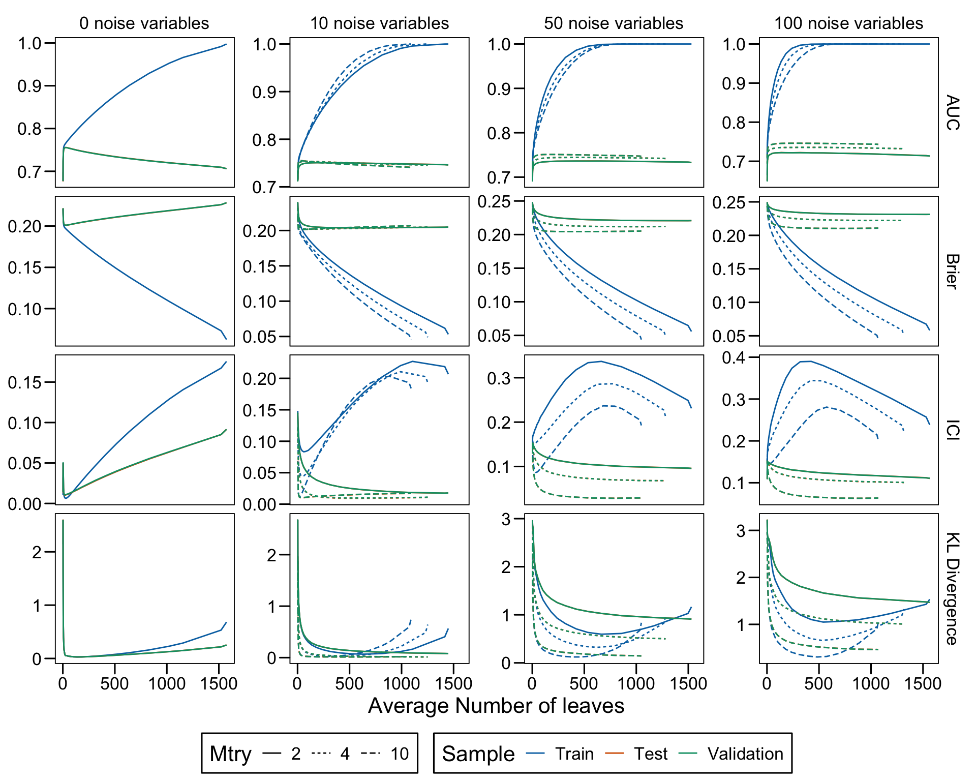
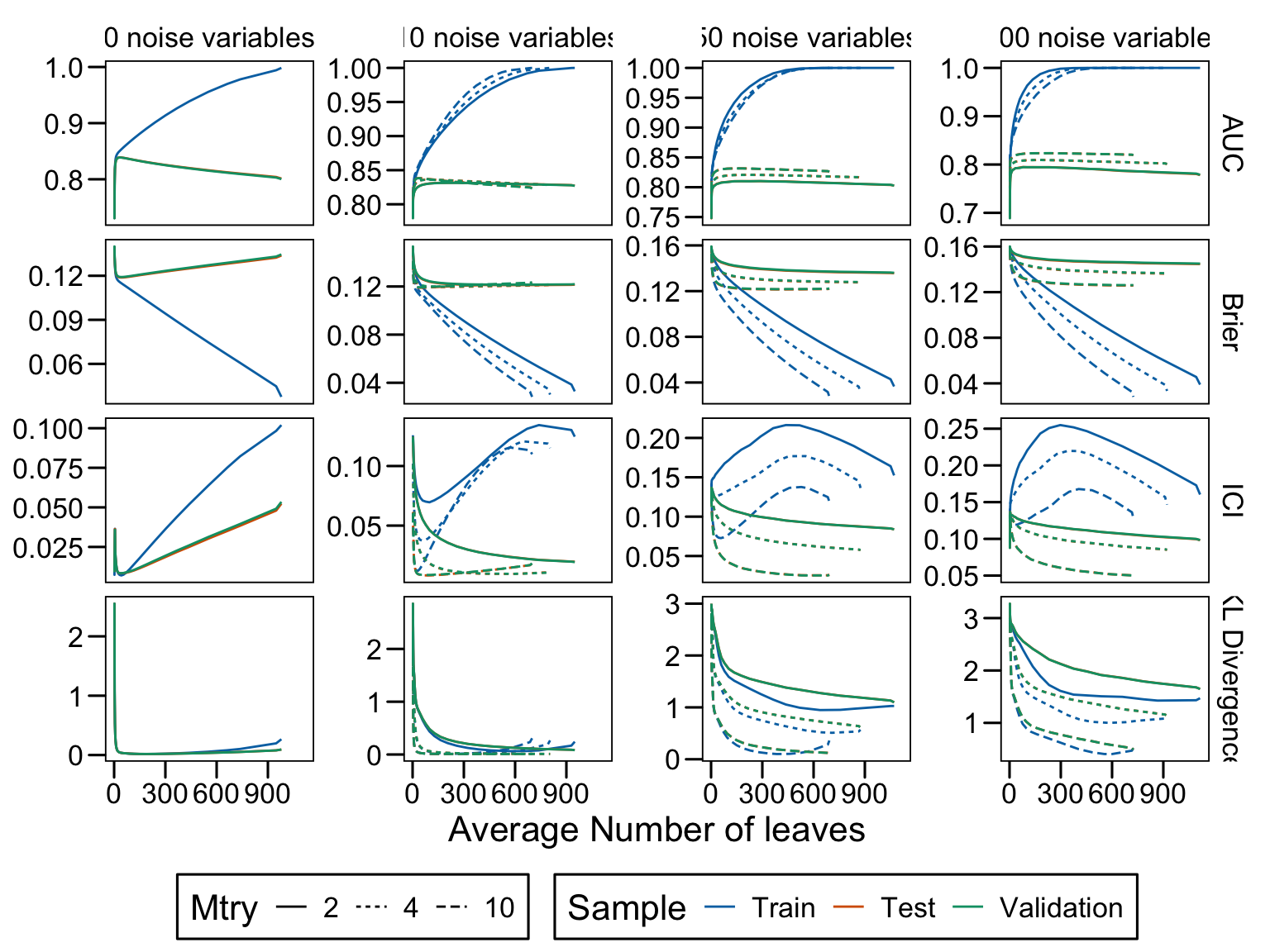
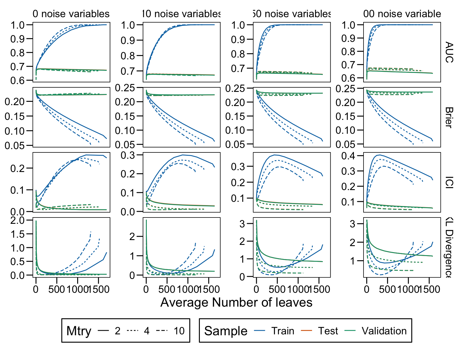
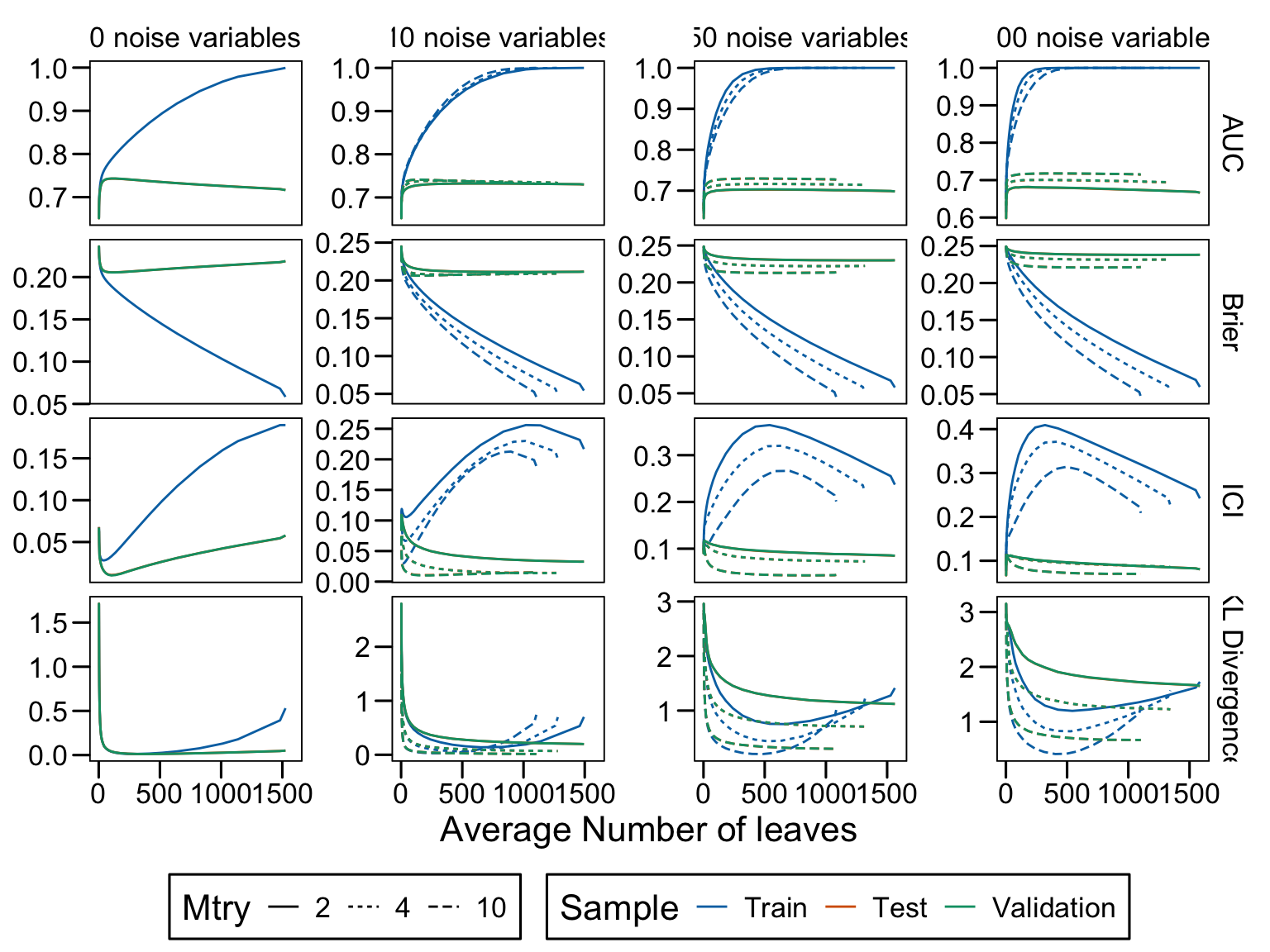
For each scenario, we train regression forests. Each forest is made of 250 trees (smaller forests are considered in Chapter 7). We consider here the following hyperparameters:

mtry: Number of variables to possibly split at in each node: 2, 4 or 10.
min_node_size: Minimal node size to split at. Varying values between 2 and 10^{4}.

min_bucket_values <- unique(round(2^seq(1, 14, by = .4)))
min_bucket_values <- min_bucket_values[min_bucket_values <=  max(params_df$size_train)]

grid <- expand_grid(
  mtry = c(2, 4, 10),
  num_trees = 250,
  min_node_size = min_bucket_values
) |> 
  mutate(ind = row_number())

The desired number of replications for each scenario needs to be set:

repns_vector <- 1:100

The different configurations are reported in Table 7.1.

Table 6.1: Grid Search Values

We define a function, simul_forest() to train a random forest on a dataset for a type of forest, with given hyperparameters (given to the function through the param argument).

Function simul_forest()

#' Train a random forest and compute performance, calibration, and dispersion 
#' metrics
#' 
#' @param params tibble with hyperparameters for the simulation
#' @param ind index of the grid (numerical ID)
#' @param simu_data simulated data obtained with `simulate_data_wrapper()`
#'  for probability trees
simul_forest <- function(params,
                         ind,
                         simu_data) {
  tb_train <- simu_data$data$train |> rename(d = y)
  tb_valid <- simu_data$data$valid |> rename(d = y)
  tb_test <- simu_data$data$test |> rename(d = y)

  true_prob <-
    list(
      train = simu_data$data$probs_train,
      valid = simu_data$data$probs_valid,
      test = simu_data$data$probs_test
    )

  ## Estimation----
  fit_rf <- ranger(
    d ~ .,
    data = tb_train,
    min.bucket = params$min_node_size,
    mtry = params$mtry,
    num.trees = params$num_trees
  )

  # Average number of leaves per trees in the forest
  nb_leaves <- map_dbl(fit_rf$forest$child.nodeIDs, ~sum(pluck(.x, 1) == 0)) |>
    mean()


  ## Raw Scores----
  # Predicted scores
  scores_train <- predict(fit_rf, data = tb_train, type = "response")$predictions
  scores_valid <- predict(fit_rf, data = tb_valid, type = "response")$predictions
  scores_test <- predict(fit_rf, data = tb_test, type = "response")$predictions

  ## Histogram of scores----
  breaks <- seq(0, 1, by = .05)
  scores_train_hist <- hist(scores_train, breaks = breaks, plot = FALSE)
  scores_valid_hist <- hist(scores_valid, breaks = breaks, plot = FALSE)
  scores_test_hist <- hist(scores_test, breaks = breaks, plot = FALSE)
  scores_hist <- list(
    train = scores_train_hist,
    valid = scores_valid_hist,
    test = scores_test_hist
  )

  ## Estimation of P(q1 < score < q2)----
  proq_scores_train <- map(
    c(.1, .2, .3, .4),
    ~prop_btw_quantiles(s = scores_train, q1 = .x)
  ) |>
    list_rbind() |>
    mutate(sample = "train")
  proq_scores_valid <- map(
    c(.1, .2, .3, .4),
    ~prop_btw_quantiles(s = scores_valid, q1 = .x)
  ) |>
    list_rbind() |>
    mutate(sample = "valid")
  proq_scores_test <- map(
    c(.1, .2, .3, .4),
    ~prop_btw_quantiles(s = scores_test, q1 = .x)
  ) |>
    list_rbind() |>
    mutate(sample = "test")

  ## Dispersion Metrics----
  disp_train <- dispersion_metrics(
    true_probas = true_prob$train, scores = scores_train
  ) |> mutate(sample = "train")

  disp_valid <- dispersion_metrics(
    true_probas = true_prob$valid, scores = scores_valid
  ) |> mutate(sample = "valid")

  disp_test <- dispersion_metrics(
    true_probas = true_prob$test, scores = scores_test
  ) |> mutate(sample = "test")

  # Performance and Calibration Metrics
  # We add very small noise to predicted scores
  # otherwise the local regression may crash
  scores_train_noise <- scores_train +
    runif(n = length(scores_train), min = 0, max = 0.01)
  scores_train_noise[scores_train_noise > 1] <- 1
  metrics_train <- compute_metrics(
    obs = tb_train$d, scores = scores_train_noise, true_probas = true_prob$train
  ) |> mutate(sample = "train")

  scores_valid_noise <- scores_valid +
    runif(n = length(scores_valid), min = 0, max = 0.01)
  scores_valid_noise[scores_valid_noise > 1] <- 1
  metrics_valid <- compute_metrics(
    obs = tb_valid$d, scores = scores_valid_noise, true_probas = true_prob$valid
  ) |> mutate(sample = "valid")

  scores_test_noise <- scores_test +
    runif(n = length(scores_test), min = 0, max = 0.01)
  scores_test_noise[scores_test_noise > 1] <- 1
  metrics_test <- compute_metrics(
    obs = tb_test$d, scores = scores_test_noise, true_probas = true_prob$test
  ) |> mutate(sample = "test")

  tb_metrics <- metrics_train |>
    bind_rows(metrics_valid) |>
    bind_rows(metrics_test) |>
    mutate(
      scenario = simu_data$scenario,
      ind = ind,
      repn = simu_data$repn,
      min_bucket = params$min_node_size,
      nb_leaves = nb_leaves,
      prop_leaves = nb_leaves / nrow(tb_train)
    )

  tb_prop_scores <- proq_scores_train |>
    bind_rows(proq_scores_valid) |>
    bind_rows(proq_scores_test) |>
    mutate(
      scenario = simu_data$scenario,
      ind = ind,
      repn = simu_data$repn,
      min_bucket = params$min_node_size,
      nb_leaves = nb_leaves,
      prop_leaves = nb_leaves / nrow(tb_train)
    )

  tb_disp_metrics <- disp_train |>
    bind_rows(disp_test) |>
    bind_rows(disp_valid) |>
    mutate(
      scenario = simu_data$scenario,
      ind = ind,
      repn = simu_data$repn,
      min_bucket = params$min_node_size,
      nb_leaves = nb_leaves,
      prop_leaves = nb_leaves / nrow(tb_train)
    )

  list(
    scenario = simu_data$scenario,     # data scenario
    ind = ind,                         # index for grid
    repn = simu_data$repn,             # data replication ID
    min_bucket = params$min_node_size, # min number of obs in terminal leaf node
    metrics = tb_metrics,              # table with performance/calib metrics
    disp_metrics = tb_disp_metrics,    # table with divergence metrics
    tb_prop_scores = tb_prop_scores,   # table with P(q1 < score < q2)
    scores_hist = scores_hist,         # histogram of scores
    nb_leaves = nb_leaves              # number of terminal leaves
  )
}

We define a wrapper function, simulate_rf_scenario() which performs a single replication of the simulations going over the different values of the grid search, for a given scenario.

Function simulate_rf_scenario()

#' Simulations for a scenario (single replication)
#' 
#' @returns list with the following elements:
#'  - `metrics_all`: computed metrics for each set of hyperparameters. 
#'    Each row gives the values for unique keys 
#'    (sample, min_bucket)
#'  - `prop_scores_simul` P(q1 < s(x) < q2) for various values of q1 and q2
#'    Each row gives the values for unique keys 
#'    (sample, min_bucket, q1, q2)
#'    q1, q2, min_bucket, type, sample)
#'  - `metrics`: computed metrics for trees of interest 
#'    (smallest, largest, largest AUC, lowest MSE, lowest KL div.).
#'    Each row gives the values for unique keys 
#'    (sample, type of tree of interest)
simulate_rf_scenario <- function(scenario, params_df, repn) {
  # Generate Data
  simu_data <- simulate_data_wrapper(
    scenario = scenario,
    params_df = params_df,
    repn = repn
  )
  
  res_simul <- vector(mode = "list", length = nrow(grid))
  # cli::cli_progress_bar("Iteration grid", total = nrow(grid), type = "tasks")
  for (j in 1:nrow(grid)) {
    curent_params <- grid |> slice(!!j)
    n_var <- simu_data$params_df$n_num + simu_data$params_df$add_categ * 5 + 
      simu_data$params_df$n_noise
    if (curent_params$mtry > n_var) {
      # cli::cli_progress_update()
      next()
    }
    
    res_simul[[j]] <- simul_forest(
      params = curent_params,
      ind = curent_params$ind,
      simu_data = simu_data
    )
    # cli::cli_progress_update()
  }
  
  metrics_simul <- map(res_simul, "metrics") |> list_rbind()
  disp_metrics_simul <- map(res_simul, "disp_metrics") |> list_rbind()
  metrics <- suppressMessages(
    left_join(metrics_simul, disp_metrics_simul)
  )
  scores_hist <- map(res_simul, "scores_hist")
  prop_scores_simul <- map(res_simul, "tb_prop_scores") |> list_rbind()
  
  # Metrics for different trees in those estimated
  # - Smallest number of leaves
  # - Largest number of leaves
  # - Max AUC
  # - Min MSE
  # - Min KL
  
  # Identify the smallest tree
  smallest <-
    metrics |>
    filter(sample == "test") |>
    arrange(nb_leaves) |>
    slice_head(n = 1) |>
    select(ind) |>
    mutate(result_type = "smallest")
  
  # Identify the largest tree
  largest <-
    metrics |>
    filter(sample == "test") |>
    arrange(desc(nb_leaves)) |>
    slice_head(n = 1) |>
    select(ind) |>
    mutate(result_type = "largest")
  
  # Identify tree with highest AUC on test set
  highest_auc <- metrics |>
    filter(sample == "test") |>
    arrange(desc(AUC)) |>
    slice_head(n = 1) |>
    select(ind) |>
    mutate(result_type = "largest_auc")
  
  # Identify tree with lowest MSE
  lowest_mse <- metrics |>
    filter(sample == "test") |>
    arrange(mse) |>
    slice_head(n = 1) |>
    select(ind) |>
    mutate(result_type = "lowest_mse")
  
  # Identify tree with lowest KL
  lowest_kl <- metrics |>
    filter(sample == "test") |>
    arrange(KL_20_true_probas) |>
    slice_head(n = 1) |>
    select(ind) |>
    mutate(result_type = "lowest_kl")
  
  trees_of_interest <-
    smallest |>
    bind_rows(largest) |>
    bind_rows(highest_auc) |>
    bind_rows(lowest_mse) |>
    bind_rows(lowest_kl)
  
  trees_of_interest_metrics <-
    trees_of_interest |>
    left_join(
      metrics, 
      by = c("ind"),
      relationship = "many-to-many" # (train, test)
    )
  trees_of_interest_prop_scores_simul <-
    trees_of_interest |>
    left_join(
      prop_scores_simul, 
      by = c("ind"),
      relationship = "many-to-many" # (train, test)
    )
  
  list(
    metrics_all = metrics,
    metrics = trees_of_interest_metrics,
    scores_hist = scores_hist,
    prop_scores_simul = trees_of_interest_prop_scores_simul
  )
}

6.4 Simulations

We loop over the scenarios and run the 100 replications in parallel.

Simulation codes

library(pbapply)
library(parallel)
ncl <- detectCores()-1
(cl <- makeCluster(ncl))

clusterEvalQ(cl, {
  library(tidyverse)
  library(philentropy)
  library(ranger)
  library(ks)
}) |> 
  invisible()

clusterExport(
  cl, c(
    # Functions
    "brier_score",
    "compute_metrics",
    "dispersion_metrics",
    "prop_btw_quantiles",
    "subset_target",
    "simulate_data",
    "simulate_data_wrapper",
    "simul_forest",
    "simulate_rf_scenario",
    # Objects
    "grid",
    "params_df",
    "repns_vector"
  )
)

dir.create("output/simul/dgp-ojeda/", recursive = TRUE)
for (i_scenario in 1:16) {
  scenario <- i_scenario
  print(str_c("Scenario ", scenario, "/", nrow(params_df)))
  clusterExport(cl, c("scenario"))
  resul_rf_scenario <-
    pblapply(
      1:length(repns_vector), function(i) simulate_rf_scenario(
        scenario = scenario, params_df = params_df, repn = repns_vector[i]
      ),
      cl = cl
    )
  save(
    resul_rf_scenario,
    file = str_c("output/simul/dgp-ojeda/resul_rf_scenario_", scenario, ".rda")
  )
}
stopCluster(cl)

The results can be loaded as follows:

files <- str_c(
  "output/simul/dgp-ojeda/resul_rf_scenario_", 1:16, ".rda"
)
resul_rf <- map(files[file.exists(files)], ~{load(.x) ; resul_rf_scenario})

The resul_rf object is of length 16: each element contains the simulations for a scenario. For each scenario, the elements are a list of length max(repns_vector), i.e., the number of replications. Each replication gives, in a list, the following elements:

metrics_all: the metrics (AUC, Calibration, KL Divergence, etc.) for each model from the grid search
scores_hist: the counts on bins defined on estimated scores (on train, validation, and test sets)
prop_scores_simul: the estimations of \(\mathbb{P}(q_1 < \hat{\mathbf{x}}< q_2)\) for various values of q_1 and q_2.

6.5 Results

We can now extract some information from the results.

6.5.1 Tables

We can merge the metrics tables computed for each scenario and replications for these scenarios into a single tibble.

metrics_rf_all <- map(
  resul_rf,
  function(resul_rf_sc) map(resul_rf_sc, "metrics_all") |> list_rbind()
) |>
  list_rbind() |>
  mutate(
    sample = factor(
      sample,
      levels = c("train", "test", "valid"),
      labels = c("Train", "Test", "Validation")
    )
  )

Let us exclude here the random forests with only 1 leaf in the nodes.

metrics_rf_all <- filter(metrics_rf_all, nb_leaves > 1)

The metrics relative to the dispersion of the scores (i.e., \(P(q_1 < \hat{s}(\mathbf{x}) < q_2)\)).

rf_prop_scores_simul <- map(
  resul_rf, 
  function(resul_rf_sc) map(resul_rf_sc, "prop_scores_simul") |> list_rbind()
) |> 
  list_rbind()

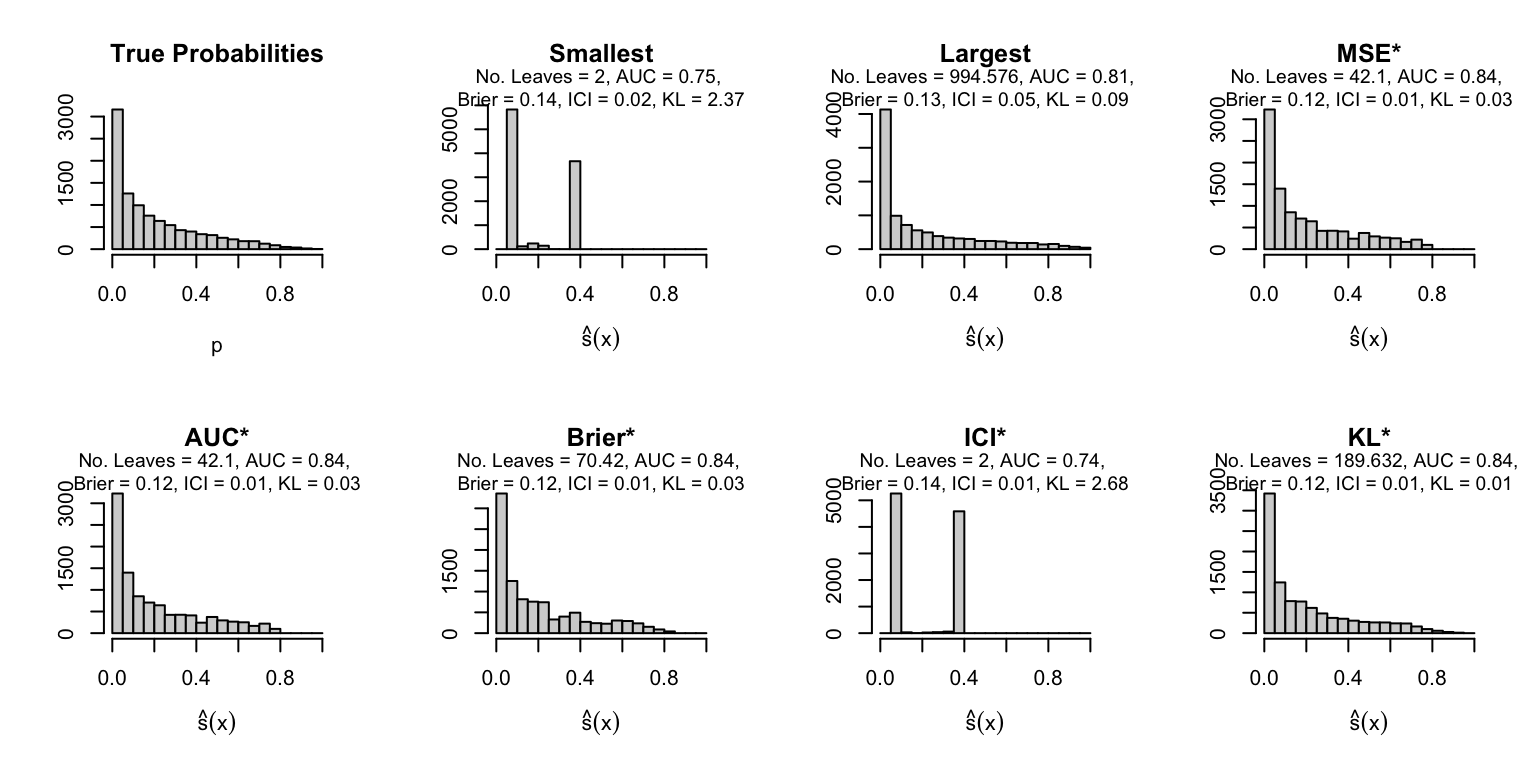
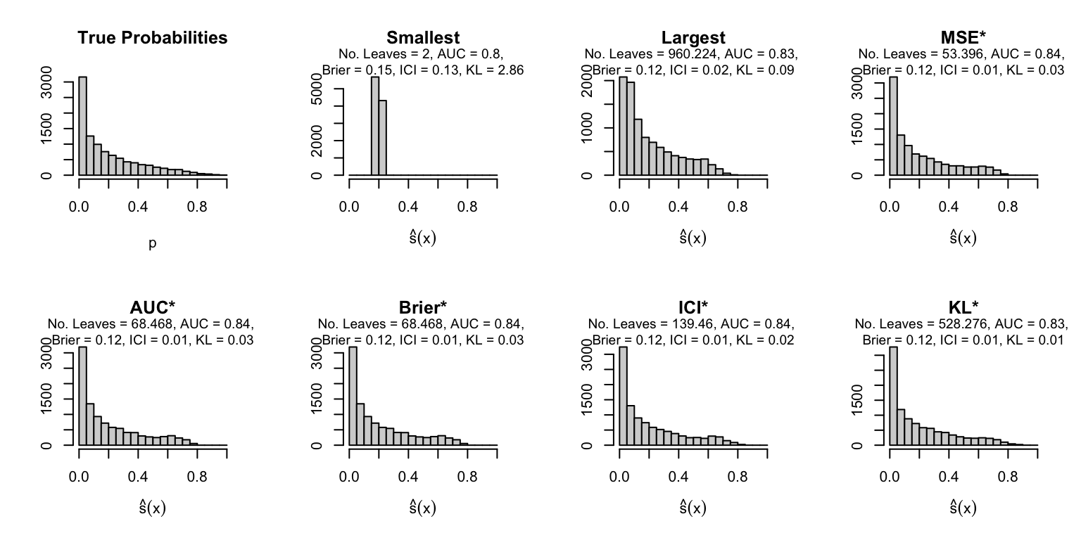
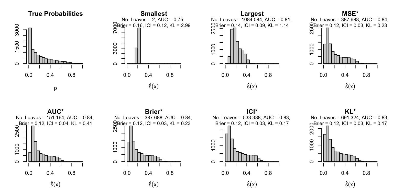
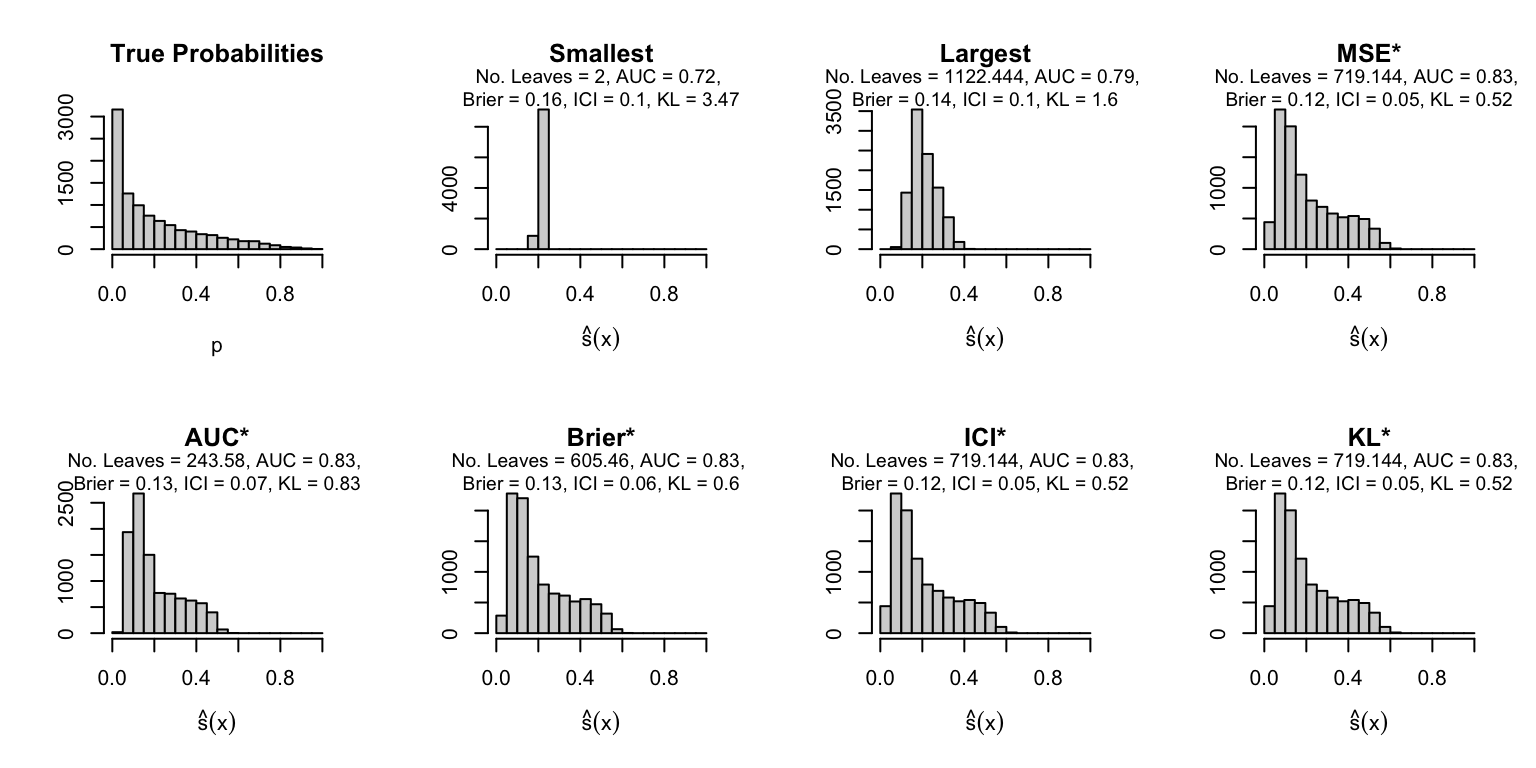
And then, let us also get the trees of interest for each replication (smallest, largest, the one that maximizes the AUC, that minimizes the MSE, that minimizes the KL divergence).

Code to identify forests of interest.

# Identify the model with the smallest number of leaves on average on
# validation set
smallest_rf <-
  metrics_rf_all |>
  filter(sample == "Validation") |>
  group_by(scenario, repn) |>
  arrange(nb_leaves) |>
  slice_head(n = 1) |>
  select(scenario, repn, ind, nb_leaves) |>
  mutate(result_type = "smallest") |>
  ungroup()

# Identify the largest tree
largest_rf <-
  metrics_rf_all |>
  filter(sample == "Validation") |>
  group_by(scenario, repn) |>
  arrange(desc(nb_leaves)) |>
  slice_head(n = 1) |>
  select(scenario, repn, ind, nb_leaves) |>
  mutate(result_type = "largest") |>
  ungroup()

# Identify tree with highest AUC on test set
highest_auc_rf <-
  metrics_rf_all |>
  filter(sample == "Validation") |>
  group_by(scenario, repn) |>
  arrange(desc(AUC)) |>
  slice_head(n = 1) |>
  select(scenario, repn, ind, nb_leaves) |>
  mutate(result_type = "largest_auc") |>
  ungroup()

# Identify tree with lowest MSE
lowest_mse_rf <-
  metrics_rf_all |>
  filter(sample == "Validation") |>
  group_by(scenario, repn) |>
  arrange(mse) |>
  slice_head(n = 1) |>
  select(scenario, repn, ind, nb_leaves) |>
  mutate(result_type = "lowest_mse") |>
  ungroup()

# Identify tree with lowest Brier
lowest_brier_rf <-
  metrics_rf_all |>
  filter(sample == "Validation") |>
  group_by(scenario, repn) |>
  arrange(brier) |>
  slice_head(n = 1) |>
  select(scenario, repn, ind, nb_leaves) |>
  mutate(result_type = "lowest_brier") |>
  ungroup()

# Identify tree with lowest ICI
lowest_ici_rf <-
  metrics_rf_all |>
  filter(sample == "Validation") |>
  group_by(scenario, repn) |>
  arrange(ici) |>
  slice_head(n = 1) |>
  select(scenario, repn, ind, nb_leaves) |>
  mutate(result_type = "lowest_ici") |>
  ungroup()

# Identify tree with lowest KL
lowest_kl_rf <-
  metrics_rf_all |>
  filter(sample == "Validation") |>
  group_by(scenario, repn) |>
  arrange(KL_20_true_probas) |>
  slice_head(n = 1) |>
  select(scenario, repn, ind, nb_leaves) |>
  mutate(result_type = "lowest_kl") |>
  ungroup()

# Merge these
rf_of_interest <-
  smallest_rf |>
  bind_rows(largest_rf) |>
  bind_rows(highest_auc_rf) |>
  bind_rows(lowest_mse_rf) |>
  bind_rows(lowest_brier_rf) |>
  bind_rows(lowest_ici_rf) |>
  bind_rows(lowest_kl_rf)

# Add metrics now
rf_of_interest <-
  rf_of_interest |>
  left_join(
    metrics_rf_all,
    by = c("scenario", "repn", "ind", "nb_leaves"),
    relationship = "many-to-many" # (train, valid, test)
  ) |>
  mutate(
    result_type = factor(
      result_type,
      levels = c(
        "smallest", "largest", "lowest_mse", "largest_auc",
        "lowest_brier", "lowest_ici", "lowest_kl"),
      labels = c(
        "Smallest", "Largest", "MSE*", "AUC*",
        "Brier*", "ICI*", "KL*"
      )
    )
  )
# Sanity check
# rf_of_interest |> count(scenario, sample, result_type)

Codes to create the table

n_digits <- 3
table_to_print <-
  rf_of_interest |>
  group_by(scenario, sample, result_type) |>
  summarise(
    across(
      all_of(c(
        "mse", "AUC", "brier", "ici", "KL_20_true_probas",
        "inter_quantile_10_90")),
      ~str_c(round(mean(.x), n_digits), " (", round(sd(.x), n_digits), ")")
    ), .groups = "drop"
  ) |>
  arrange(scenario, result_type) |>
  mutate(scenario = str_c("Scenario ", scenario))

table_to_print |>
  DT::datatable(
    rownames = FALSE,
    colnames = c(
      "Scenario" = "scenario",
      "Selected Tree" = "result_type",
      "Sample" = "sample",
      "ICI" = "ici",
      "KL Div." = "KL_20_true_probas",
      "Quant. Ratio" = "inter_quantile_10_90"
    ),
    filter = "top",
    extensions = 'RowGroup',
    options = list(
      rowGroup = list(dataSrc = c(0)),
      iDisplayLength = 21
    )
  ) |>
  DT::formatStyle(
    1:ncol(table_to_print),
    target = 'row',
    backgroundColor = DT::styleEqual(
      c("Smallest", "Largest", "AUC*", "MSE*", "Brier*", "ICI*", "KL*"),
      c("#332288", "#117733", "#AA4499", "#882255","#DDCC77", "#44AA99", "#949698")
    ),
    color = "white"
  )

Table 6.2: Average Performance and Calibration Metrics Computed on Test Set Over 100 Replications Under Scenario 1. Standard errors between round brackets.

6.5.2 Figures

6.5.2.1 Scores Distributions

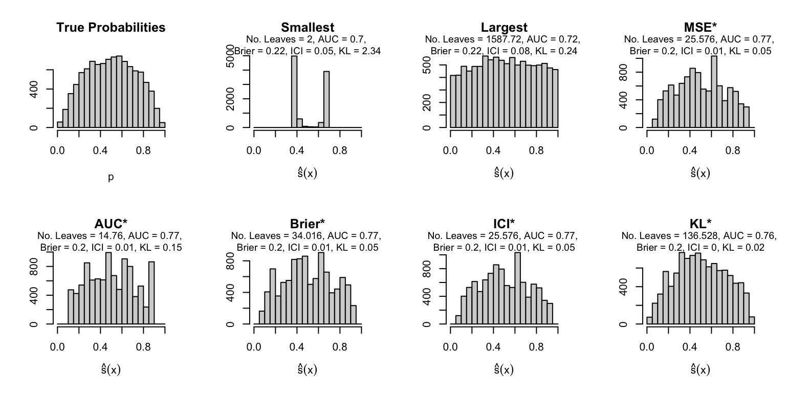
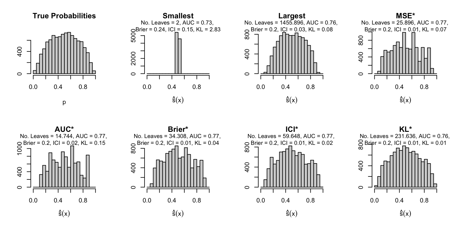
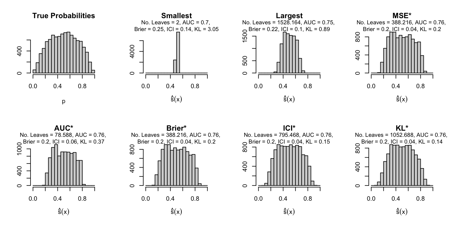
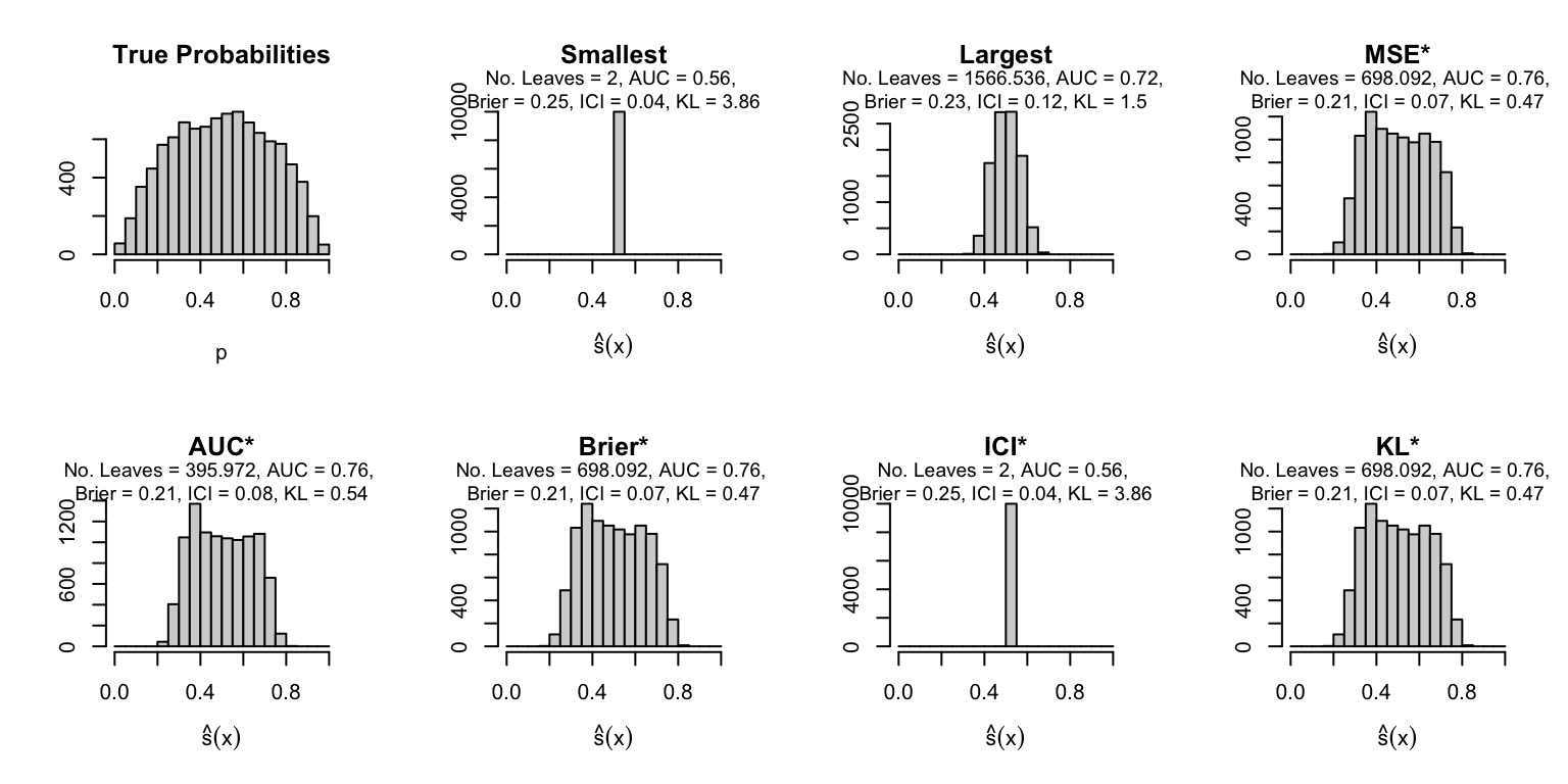
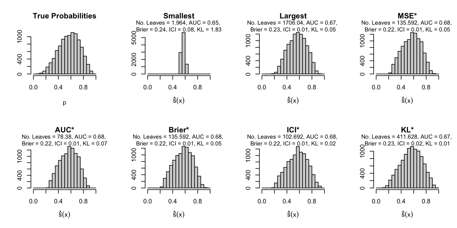
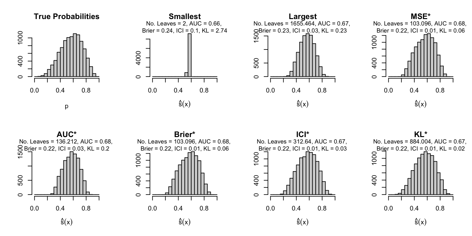
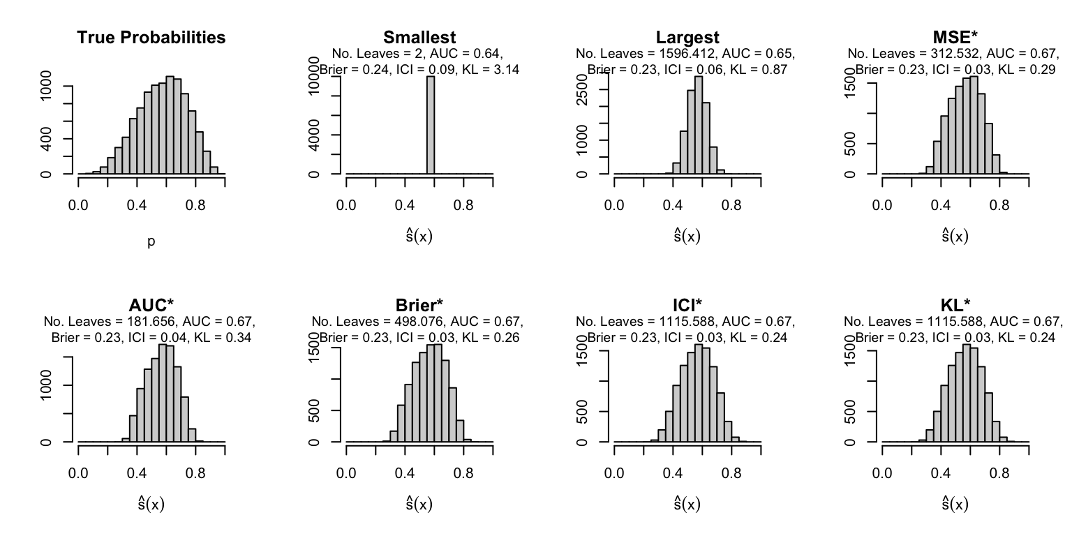
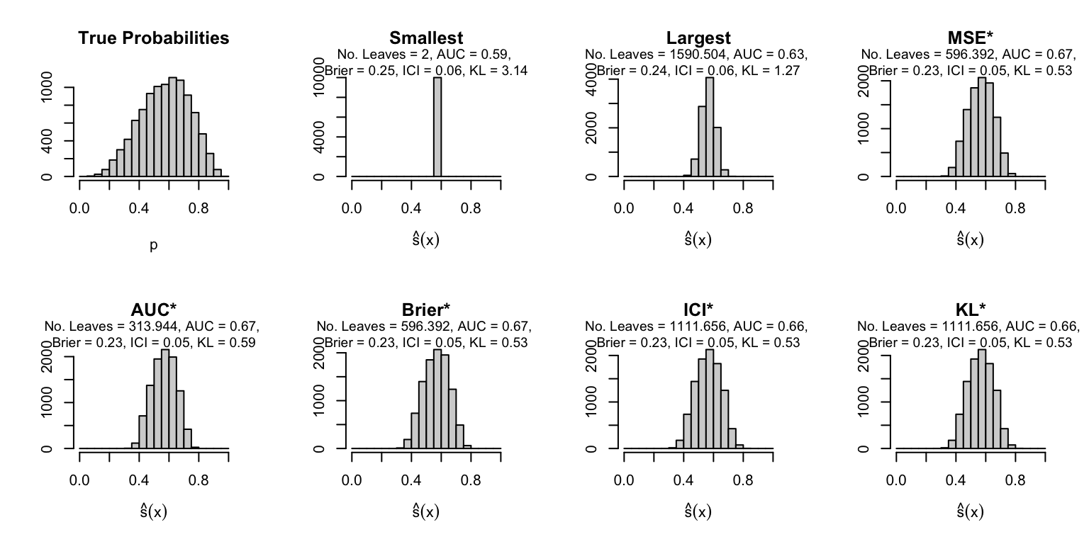
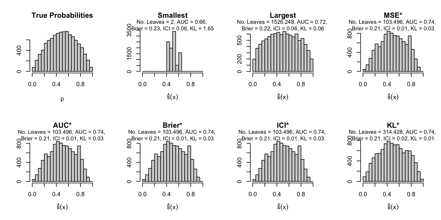
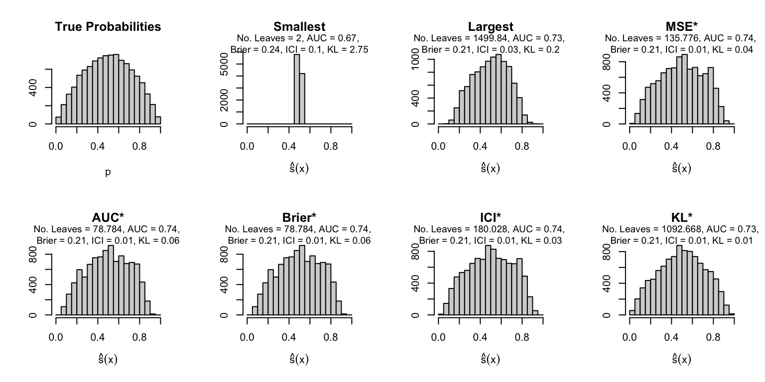
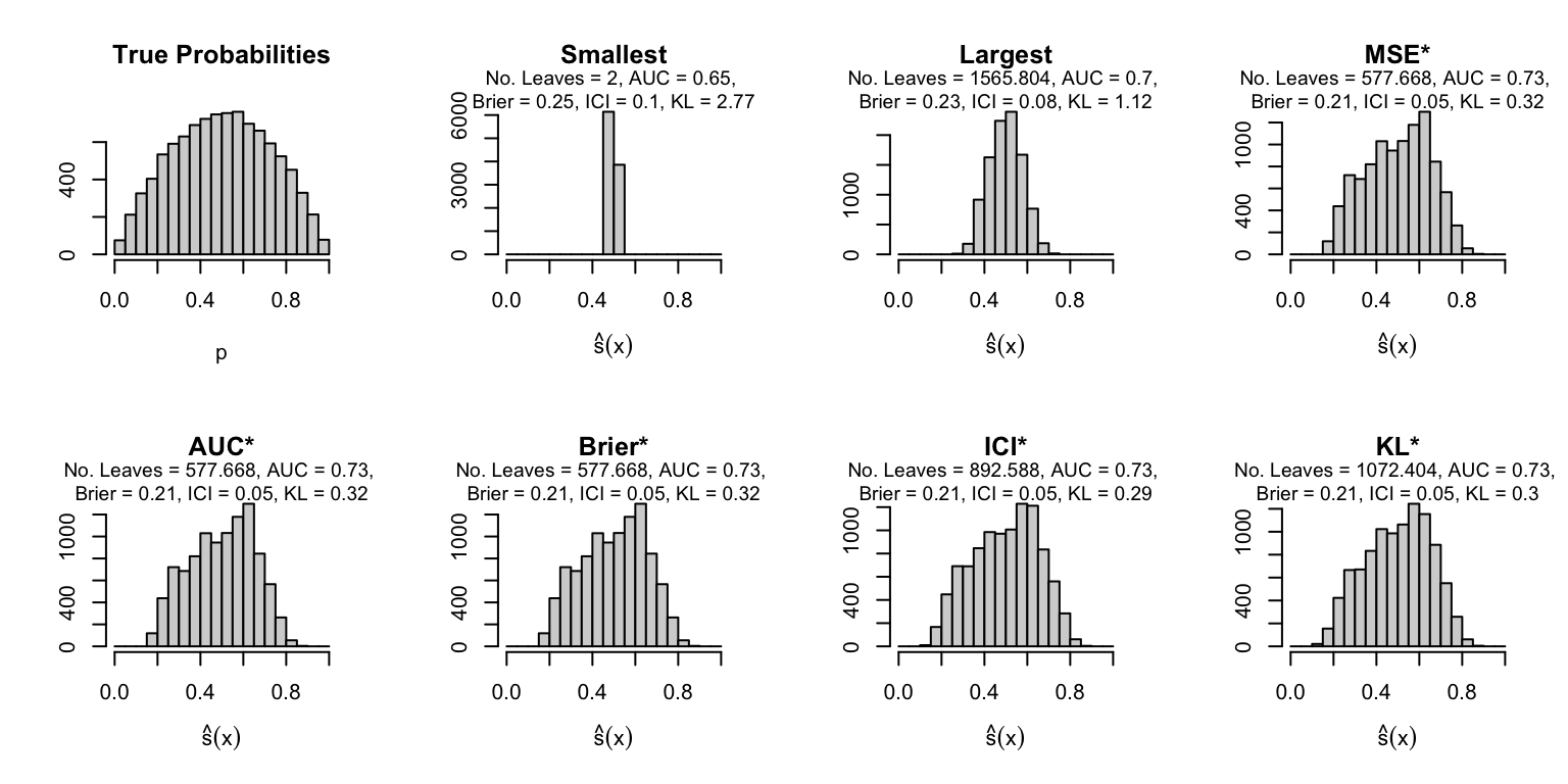
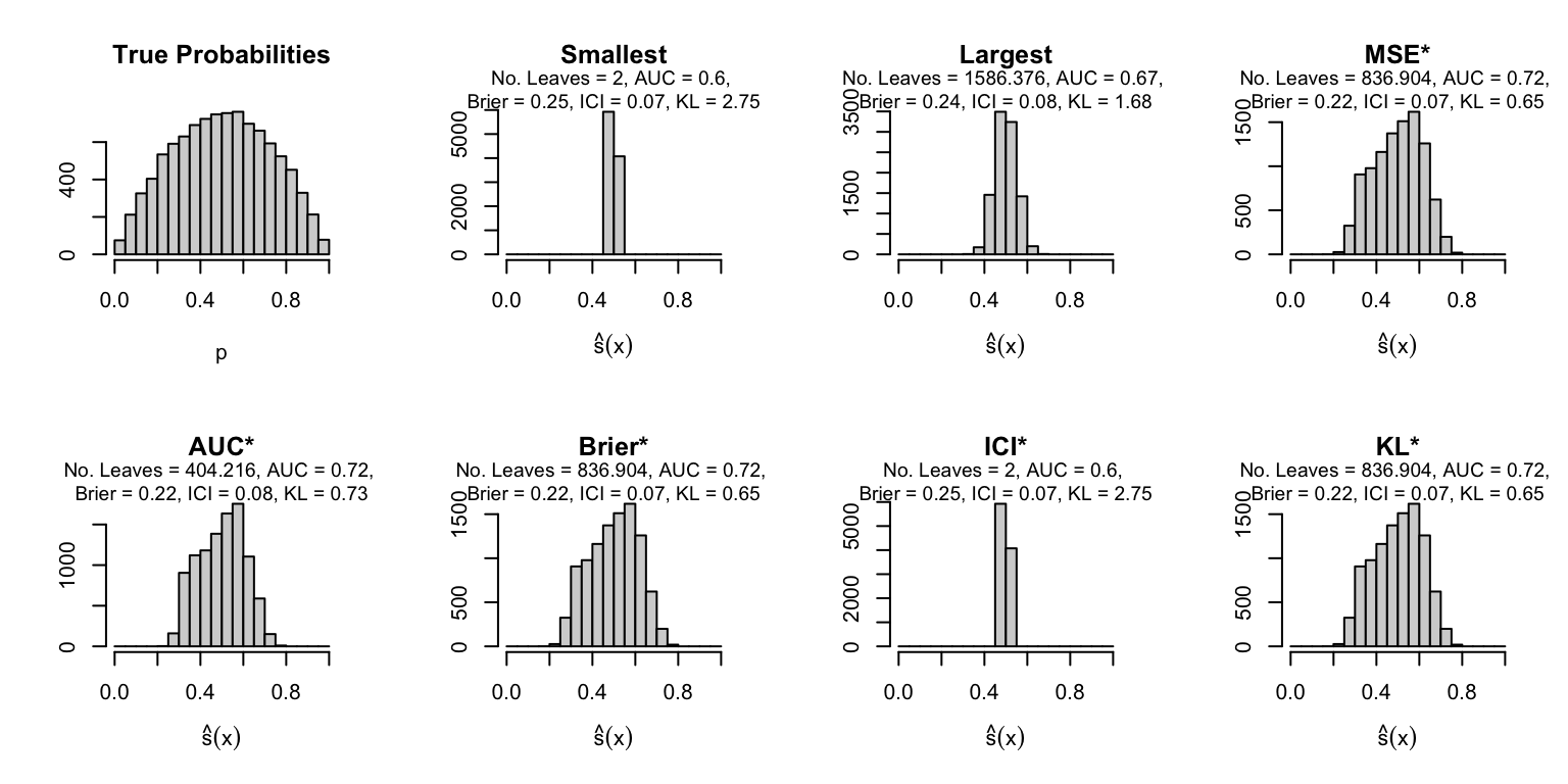
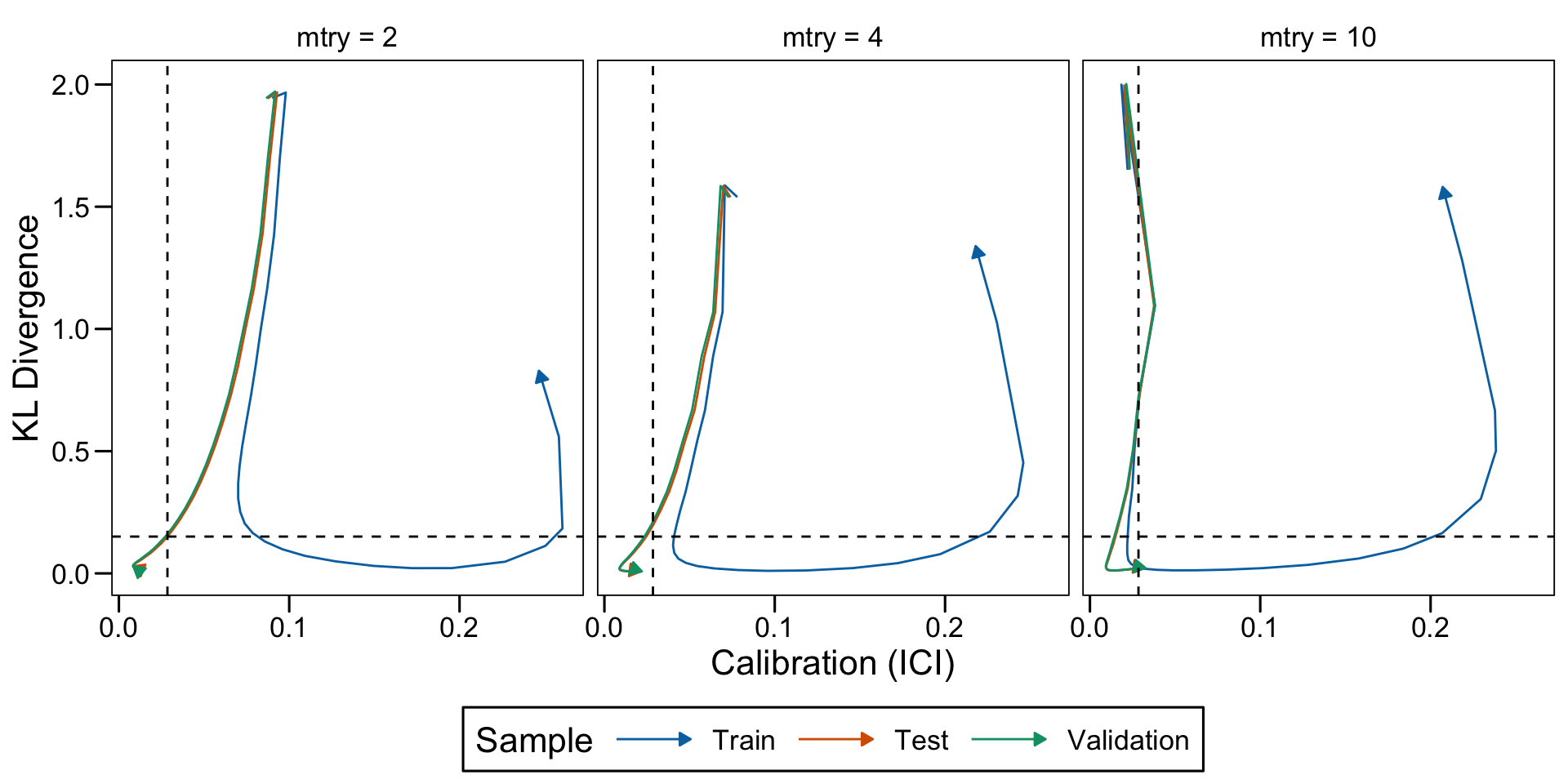
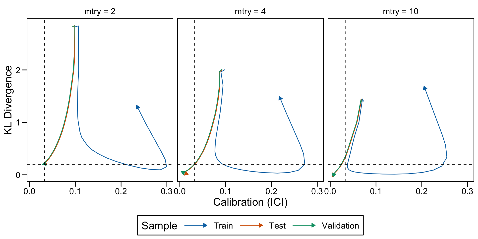
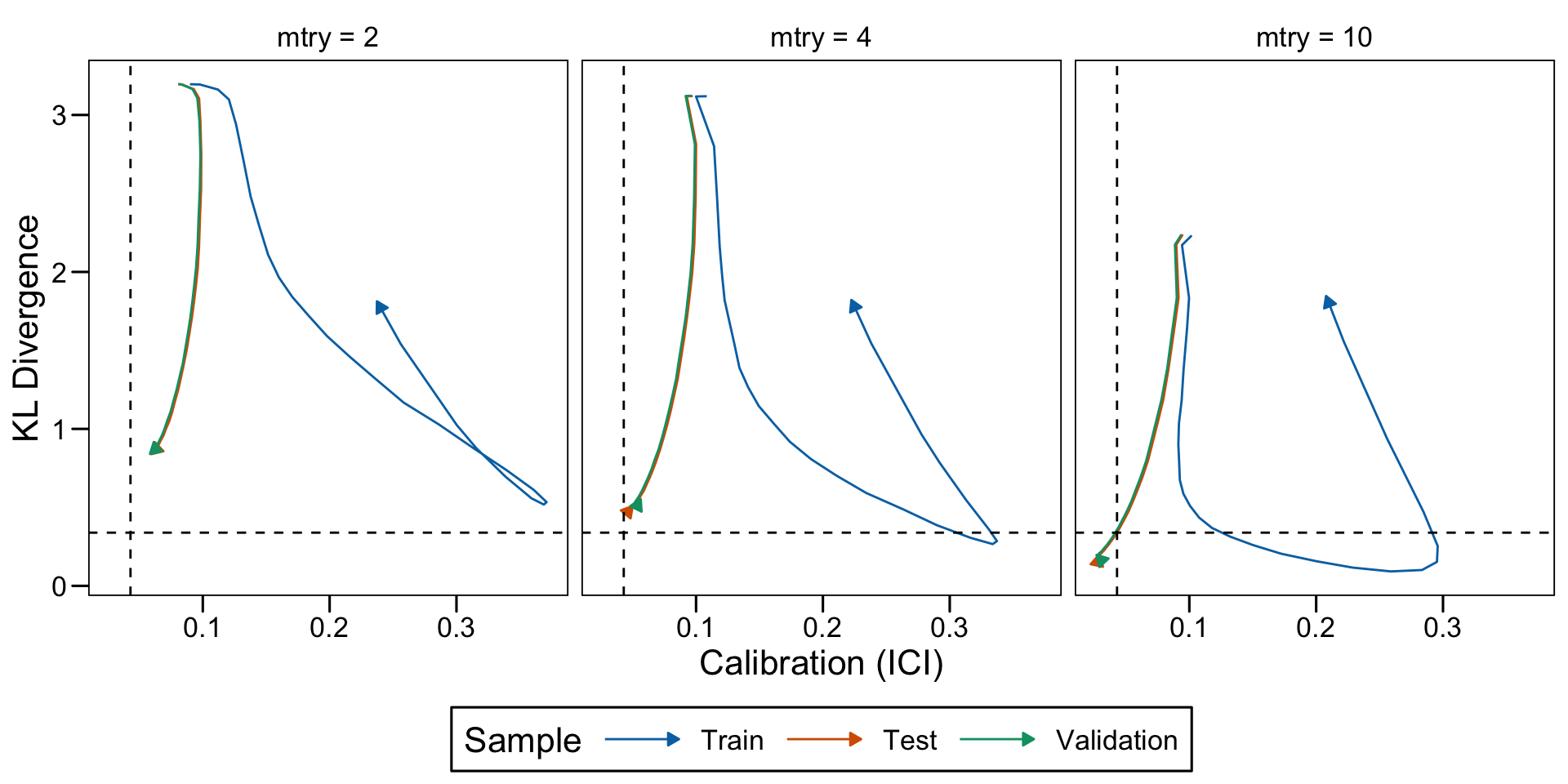
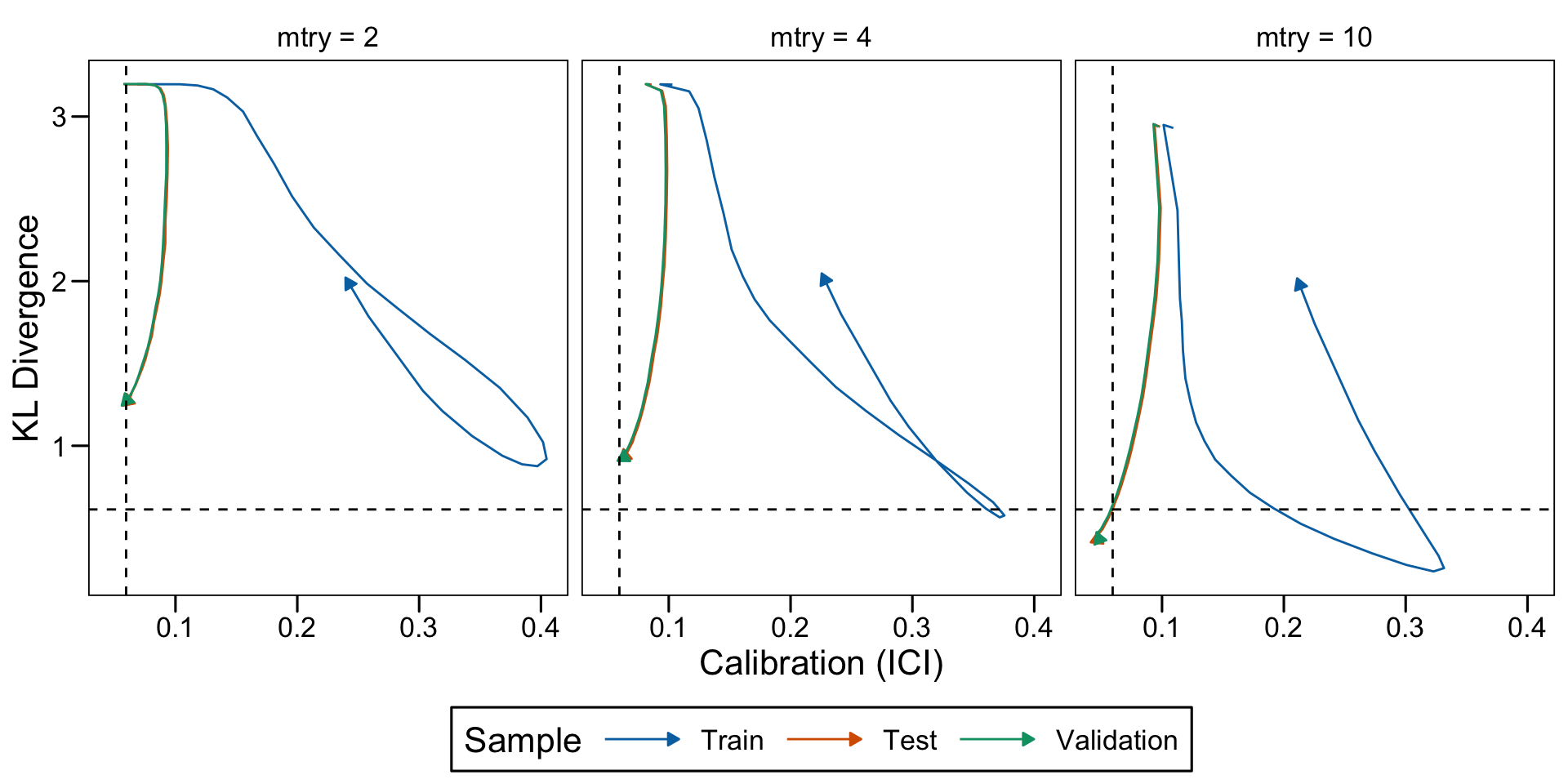
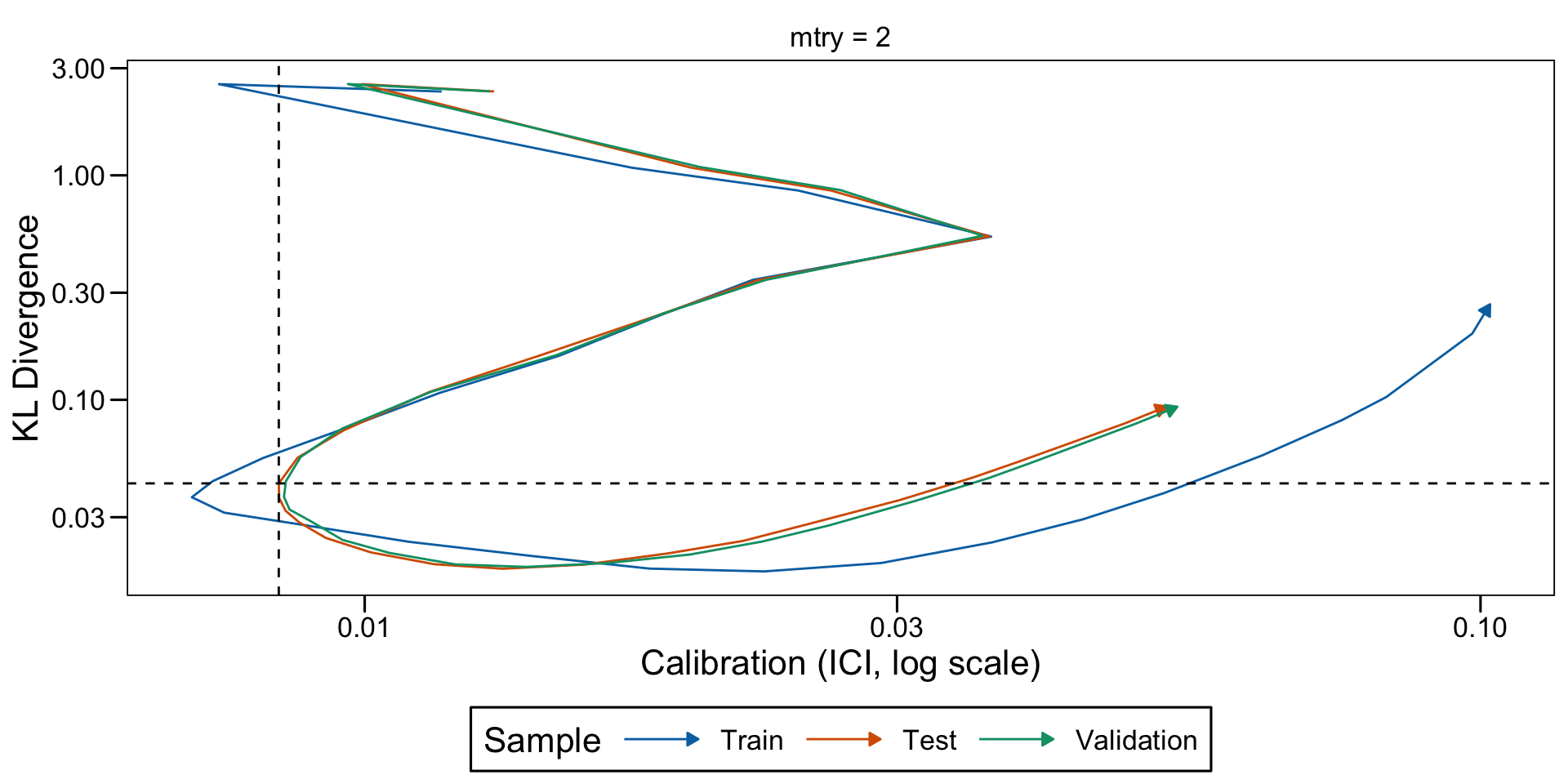
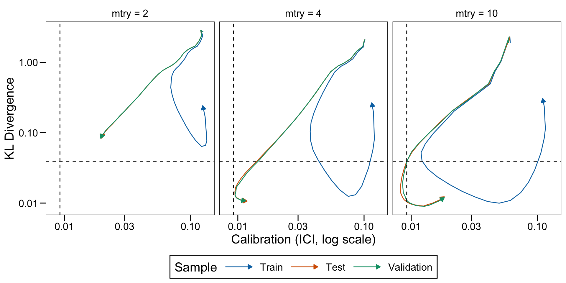
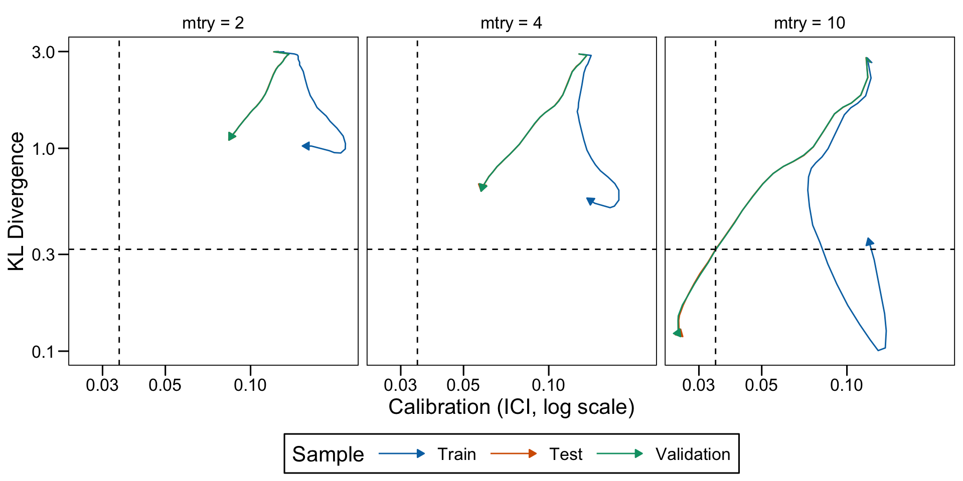
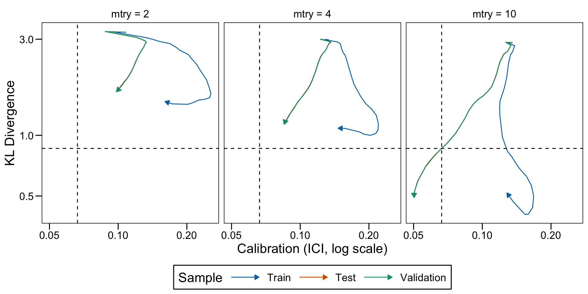
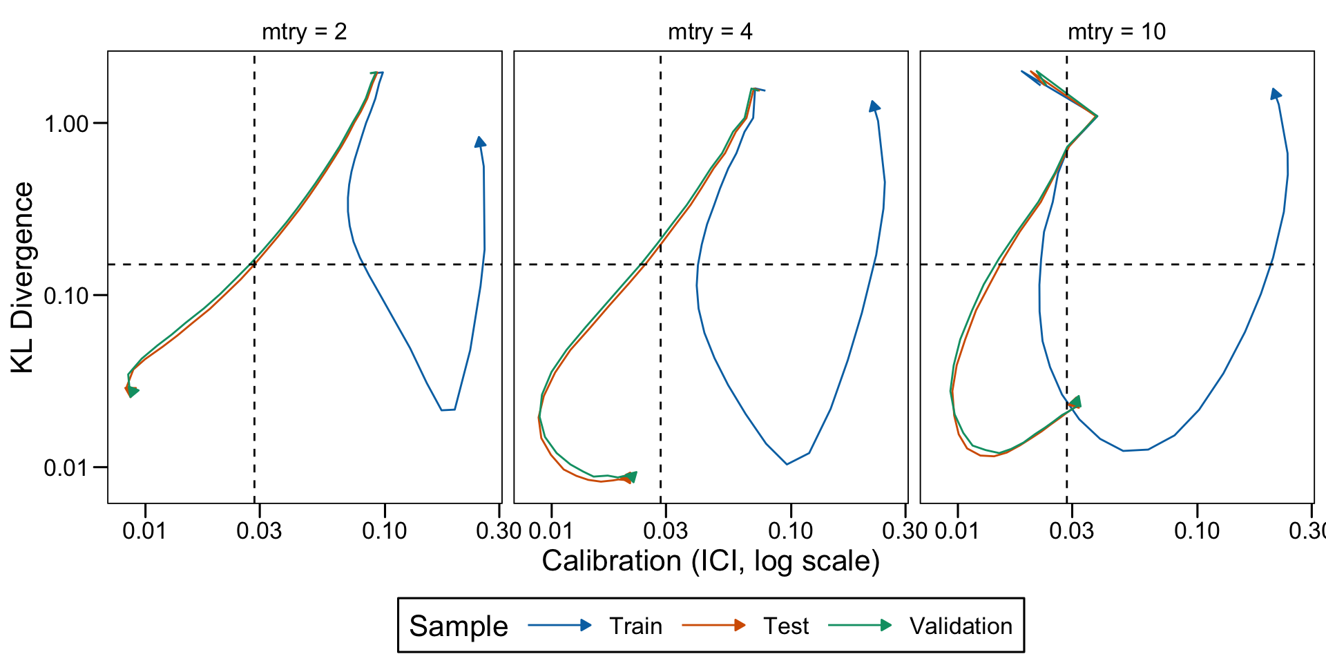
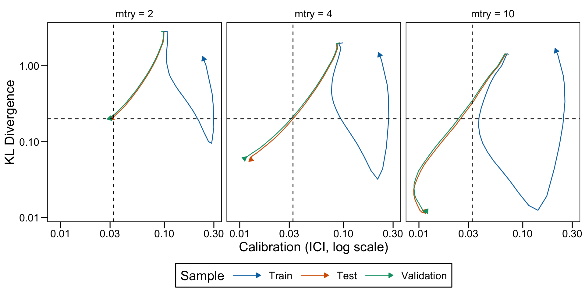
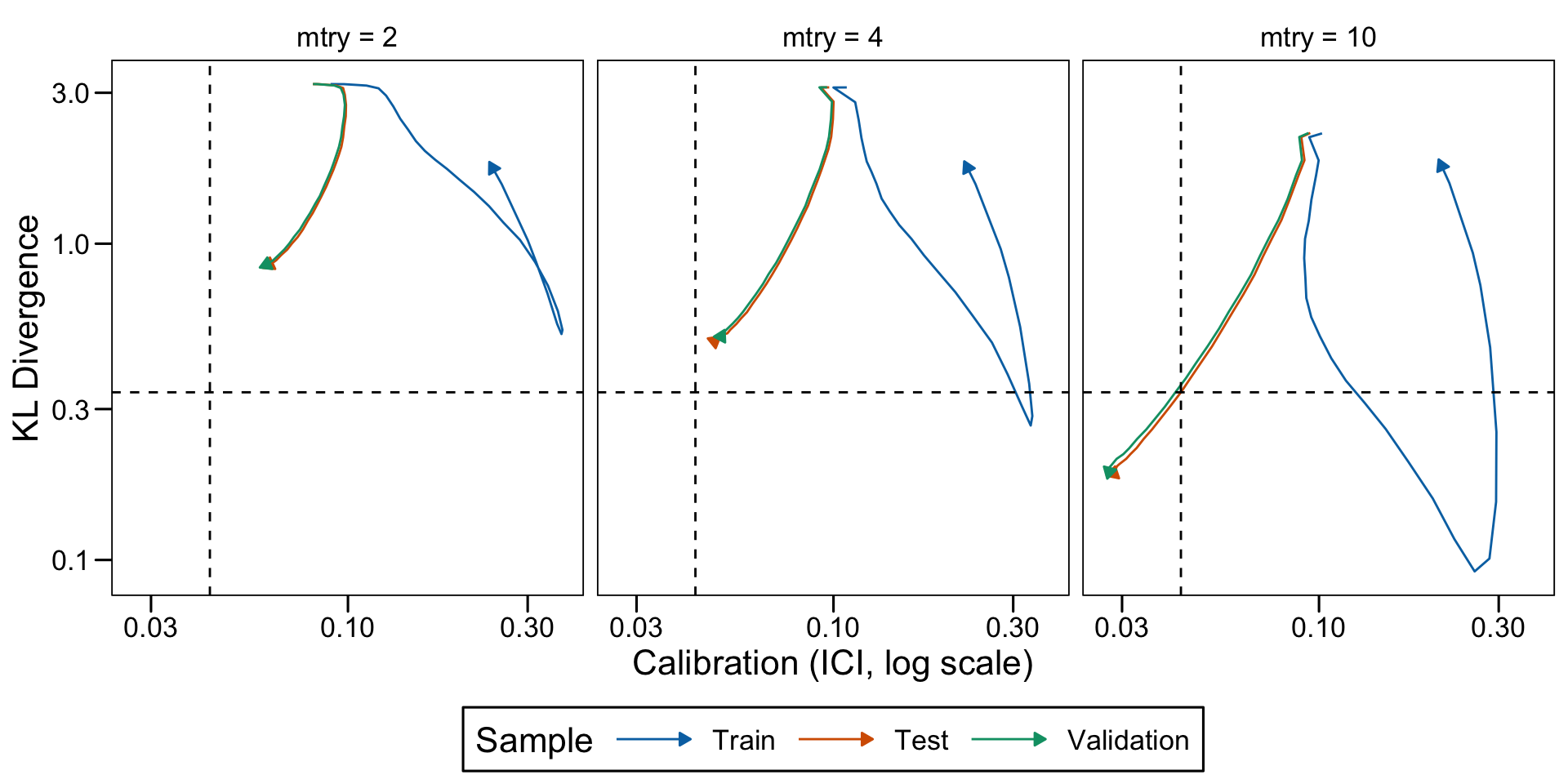
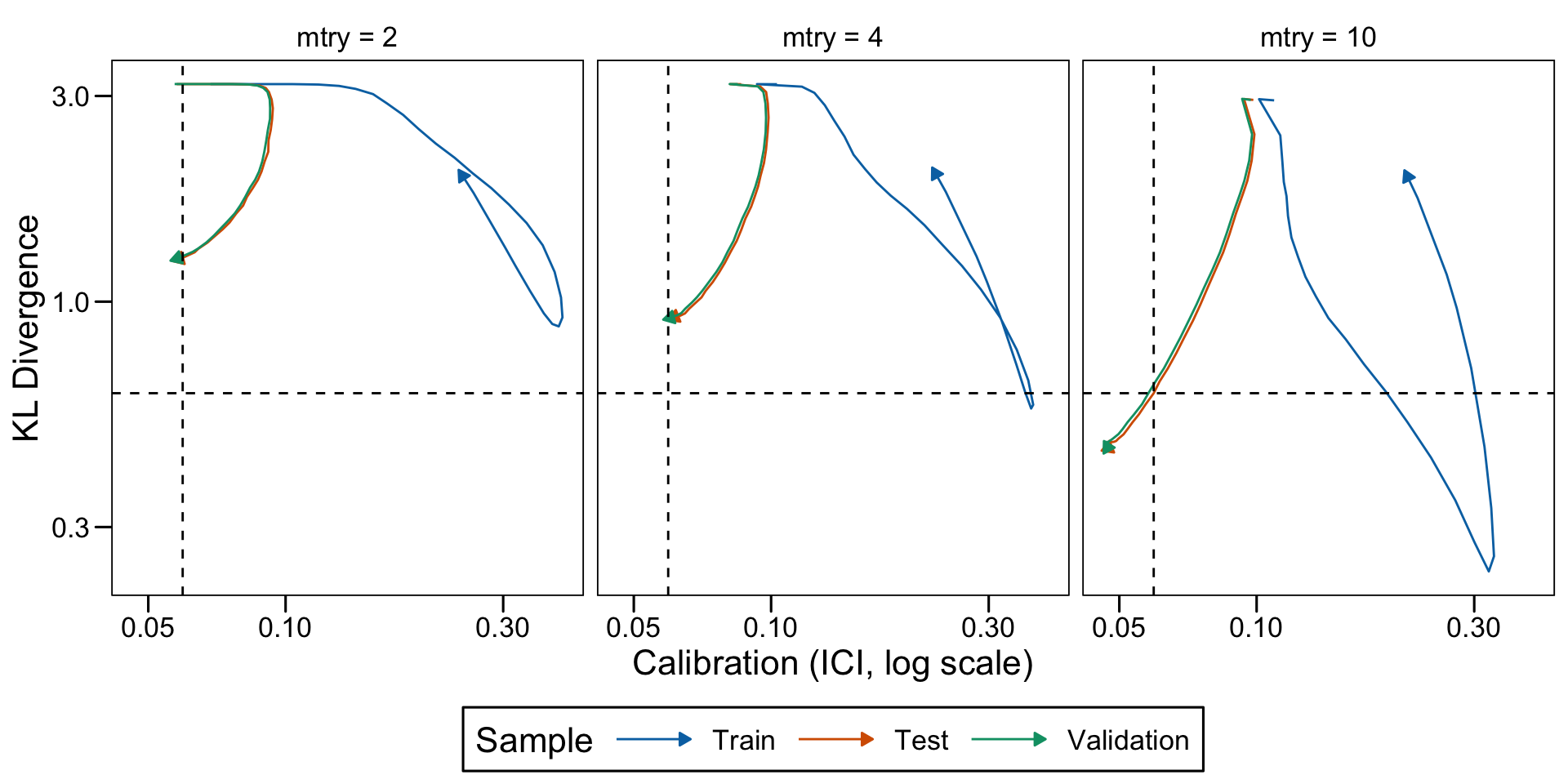
Let us plot the distributions of scores for the trees of interest (smallest, largest, max AUC, min MSE, min KL) for a single replication (the first replication) for each scenario.

Codes to get the barplots

get_bp <- function(interest,
                   scenario,
                   repn) {
  # Identify the row number of the grid
  rf_of_interest_plot <-
    rf_of_interest |>
    filter(
      result_type == !!interest,
      scenario == !!scenario,
      repn == !!repn,
      sample == "Test"
    )

  ind_grid <- rf_of_interest_plot |>
    pull("ind")

  # The corresponding barplots data
  data_bp <-
    map(resul_rf[[scenario]], "scores_hist")[[repn]] |>
    pluck(ind_grid)

  subtitle <- str_c(
    "No. Leaves = ", rf_of_interest_plot$nb_leaves, ", ",
    "AUC = ", round(rf_of_interest_plot$AUC, 2), ", \n",
    "Brier = ", round(rf_of_interest_plot$brier, 2), ", ",
    "ICI = ", round(rf_of_interest_plot$ici, 2), ", ",
    "KL = ", round(rf_of_interest_plot$KL_20_true_probas, 2)
  )

  plot(
    main = interest,
    data_bp$test,
    xlab = latex2exp::TeX("$\\hat{s}(x)$"),
    ylab = ""
  )
  mtext(side = 3, line = -0.25, adj = .5, subtitle, cex = .6)
}

plot_hist_scenario <- function(scenario,
                               repn) {
  par(mfrow = c(2,4))
  # True probabilities
  simu_data <- simulate_data_wrapper(
    scenario = scenario,
    params_df = params_df,
    repn = repn # only one replication here
  )
  true_prob <- simu_data$data$probs_train
  hist(
    true_prob,
    breaks = seq(0, 1, by = .05),
    xlab = "p", ylab = "",
    main = "True Probabilities",
    xlim = c(0, 1)
  )

  for (interest in c("Smallest", "Largest", "MSE*" ,
                     "AUC*", "Brier*", "ICI*", "KL*")) {
    get_bp(
      interest = interest,
      scenario = scenario,
      repn = repn
    )
  }
}

Showing plots for the first replication only:

repn <- 1

Distribution of true probabilities and estimated scores on test set for random forests of interest (DGP 1, 0 noise variables)

Distribution of true probabilities and estimated scores on test set for random forests of interest (DGP 1, 10 noise variables)

Distribution of true probabilities and estimated scores on test set for random forests of interest (DGP 1, 50 noise variables)

Distribution of true probabilities and estimated scores on test set for random forests of interest (DGP 1, 100 noise variables)

Distribution of true probabilities and estimated scores on test set for random forests of interest (DGP 2, 0 noise variables)

Distribution of true probabilities and estimated scores on test set for random forests of interest (DGP 2, 10 noise variables)

Distribution of true probabilities and estimated scores on test set for random forests of interest (DGP 2, 50 noise variables)

Distribution of true probabilities and estimated scores on test set for random forests of interest (DGP 2, 100 noise variables)

Distribution of true probabilities and estimated scores on test set for random forests of interest (DGP 3, 0 noise variables)

Distribution of true probabilities and estimated scores on test set for random forests of interest (DGP 3, 10 noise variables)

Distribution of true probabilities and estimated scores on test set for random forests of interest (DGP 3, 50 noise variables)

Distribution of true probabilities and estimated scores on test set for random forests of interest (DGP 3, 100 noise variables)

Distribution of true probabilities and estimated scores on test set for random forests of interest (DGP 4, 0 noise variables)

Distribution of true probabilities and estimated scores on test set for random forests of interest (DGP 4, 10 noise variables)

Distribution of true probabilities and estimated scores on test set for random forests of interest (DGP 4, 50 noise variables)

Distribution of true probabilities and estimated scores on test set for random forests of interest (DGP 4, 100 noise variables)

6.5.2.2 Metrics vs Number of Leaves

We can also plot some metrics as a function of the average number of leaves in the trees of the forests.

Codes to get the plots

plot_metric_leaves <- function(dgp) {
  data_plot <-
    metrics_rf_all |>
    mutate(
      dgp = case_when(
        scenario %in% 1:4 ~ 1,
        scenario %in% 5:8 ~ 2,
        scenario %in% 9:12 ~ 3,
        scenario %in% 13:16 ~ 4
      ),
      no_noise = c(0, 10, 50, 100)[(scenario-1)%%4 + 1],
      no_noise = factor(no_noise, levels = c(no_noise), labels = str_c(no_noise, " noise variables"))
    ) |>
    filter(dgp == !!dgp) |>
    left_join(grid |> select(ind, mtry, min_node_size, num_trees), by = "ind") |>
    group_by(
      sample, dgp, no_noise, scenario, ind, mtry
    ) |>
    summarise(
      KL_20_true_probas = mean(KL_20_true_probas),
      auc = mean(AUC),
      brier = mean(brier),
      ici = mean(ici),
      nb_leaves = mean(nb_leaves),
      .groups = "drop"
    ) |>
    mutate(
      mtry_lab = factor(mtry),
      mtry_lab = fct_reorder(mtry_lab, mtry),
    ) |>
    pivot_longer(cols = c(auc, brier, ici, KL_20_true_probas), names_to = "metric") |>
    mutate(metric = factor(
      metric,
      levels = c("auc", "brier", "ici", "KL_20_true_probas"),
      labels = c("AUC", "Brier", "ICI", "KL Divergence")
    ))

  ggplot(
    data = data_plot |> group_by(mtry_lab) |> arrange(nb_leaves),
    mapping = aes(x = nb_leaves, y = value)
  ) +
    geom_line(
      mapping = aes(colour = sample, linetype = mtry_lab, group = )
    ) +
    ggh4x::facet_grid2(metric~no_noise, scales = "free_y", independent = "y") +
    scale_colour_manual("Sample", values = colour_samples) +
    scale_linetype_discrete("Mtry") +
    theme_paper() +
    labs(x = "Average Number of leaves", y = NULL)
}

Code

plot_metric_leaves(dgp = 1)

Metrics depending on the average number of leaves in the estimated trees of the forests (DGP 1)

Code

plot_metric_leaves(dgp = 2)

Metrics depending on the average number of leaves in the estimated trees of the forests (DGP 2)

Code

plot_metric_leaves(dgp = 3)

Metrics depending on the average number of leaves in the estimated trees of the forests (DGP 3)

Code

plot_metric_leaves(dgp = 4)

Metrics depending on the average number of leaves in the estimated trees of the forests (DGP 4)

6.5.2.3 Relationship between calibration, KL divergence and tree complexity

For a given scenario, each dot in the figures below is obtained by computing the average metrics on the 100 replications.

Codes to get the plots

plot_kl_vs_calib <- function(scenario_number,
                             calib_metric,
                             log_scale = FALSE) {
  data_plot <- metrics_rf_all |>
    left_join(grid |> select(ind, mtry)) |>
    filter(scenario == !!scenario_number) |>
    group_by(
      sample, scenario, ind, mtry
    ) |>
    summarise(
      KL_20_true_probas = mean(KL_20_true_probas),
      ici = mean(ici),
      brier = mean(brier),
      nb_leaves = mean(nb_leaves),
      auc = mean(AUC),
      .groups = "drop"
    ) |>
    mutate(
      mtry_lab = factor(str_c("mtry = ", mtry)),
      mtry_lab = fct_reorder(mtry_lab, mtry)
    )


  data_plot_max_auc <-
    data_plot |>
    filter(sample == "Test") |>
    group_by(sample, scenario) |> # not by mtry here
    mutate(is_max_auc = auc == max(auc)) |>
    ungroup() |>
    filter(is_max_auc == TRUE) |>
    select(sample, scenario, !!calib_metric, KL_20_true_probas)

  x_lab <- str_c(
    "Calibration (", ifelse(calib_metric == "ici", "ICI", "Brier Score"),
    ifelse(log_scale == TRUE, ", log scale)", ")")
  )


  p <- ggplot(
    data = data_plot |> group_by(mtry) |> arrange(nb_leaves),
    mapping = aes(
      x = !!sym(calib_metric), y = KL_20_true_probas
    )
  ) +
    # geom_point(alpha = .5, mapping = aes(size = nb_leaves, colour = sample)) +
    geom_path(
      mapping = aes(colour = sample),
      arrow = arrow(type = "closed", ends = "last",
                    length = unit(0.08, "inches"))
    ) +
    geom_vline(
      data = data_plot_max_auc,
      mapping = aes(xintercept = !!sym(calib_metric)),
      linetype = "dashed"
    ) +
    geom_hline(
      data = data_plot_max_auc,
      mapping = aes(yintercept = KL_20_true_probas),
      linetype = "dashed"
    ) +
    facet_grid(~mtry_lab) +
    scale_colour_manual("Sample", values = colour_samples) +
    labs(x = x_lab, y = "KL Divergence") +
    scale_size_binned_area("Number of Leaves") +
    theme_paper() +
    theme(legend.key.width = unit(1.5, "cm"))

  if (log_scale) p <- p + scale_x_log10() + scale_y_log10()
  p
}

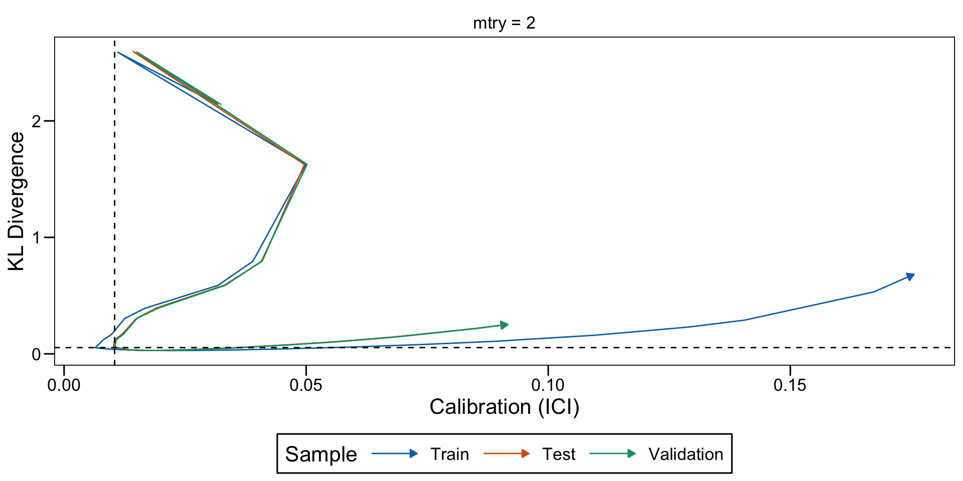
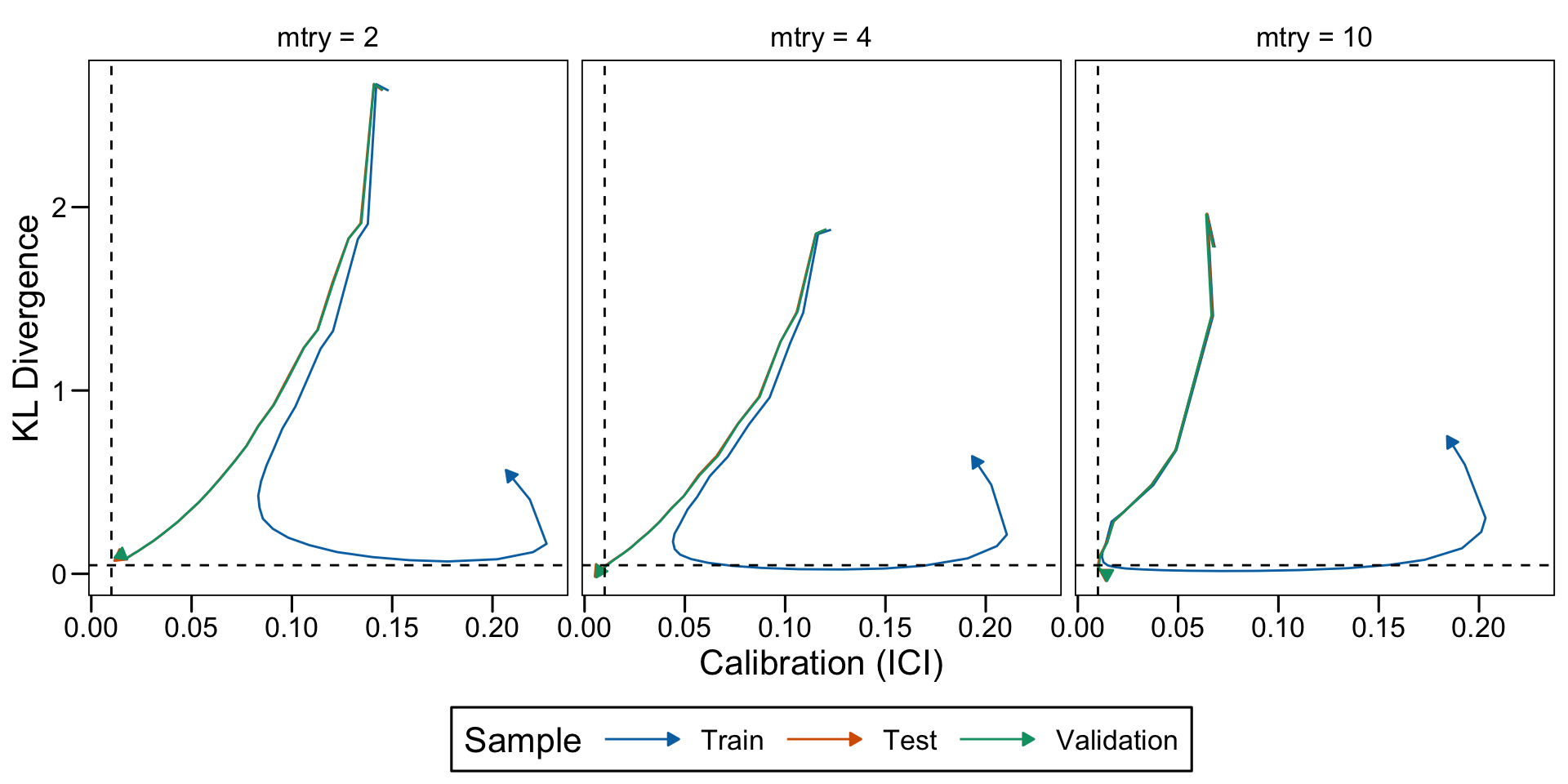
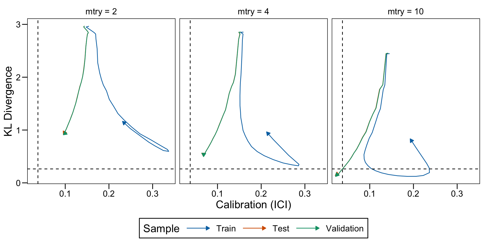
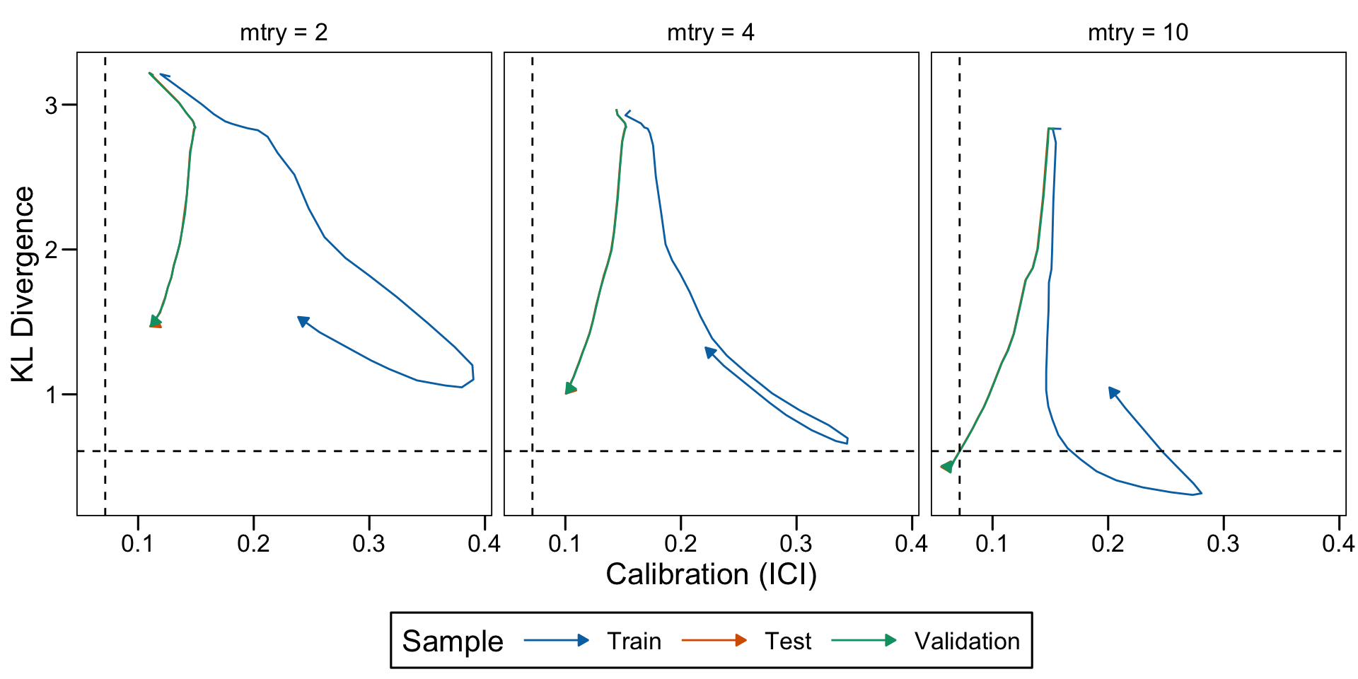
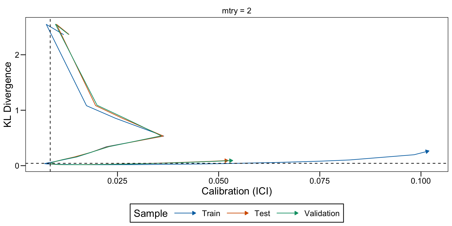
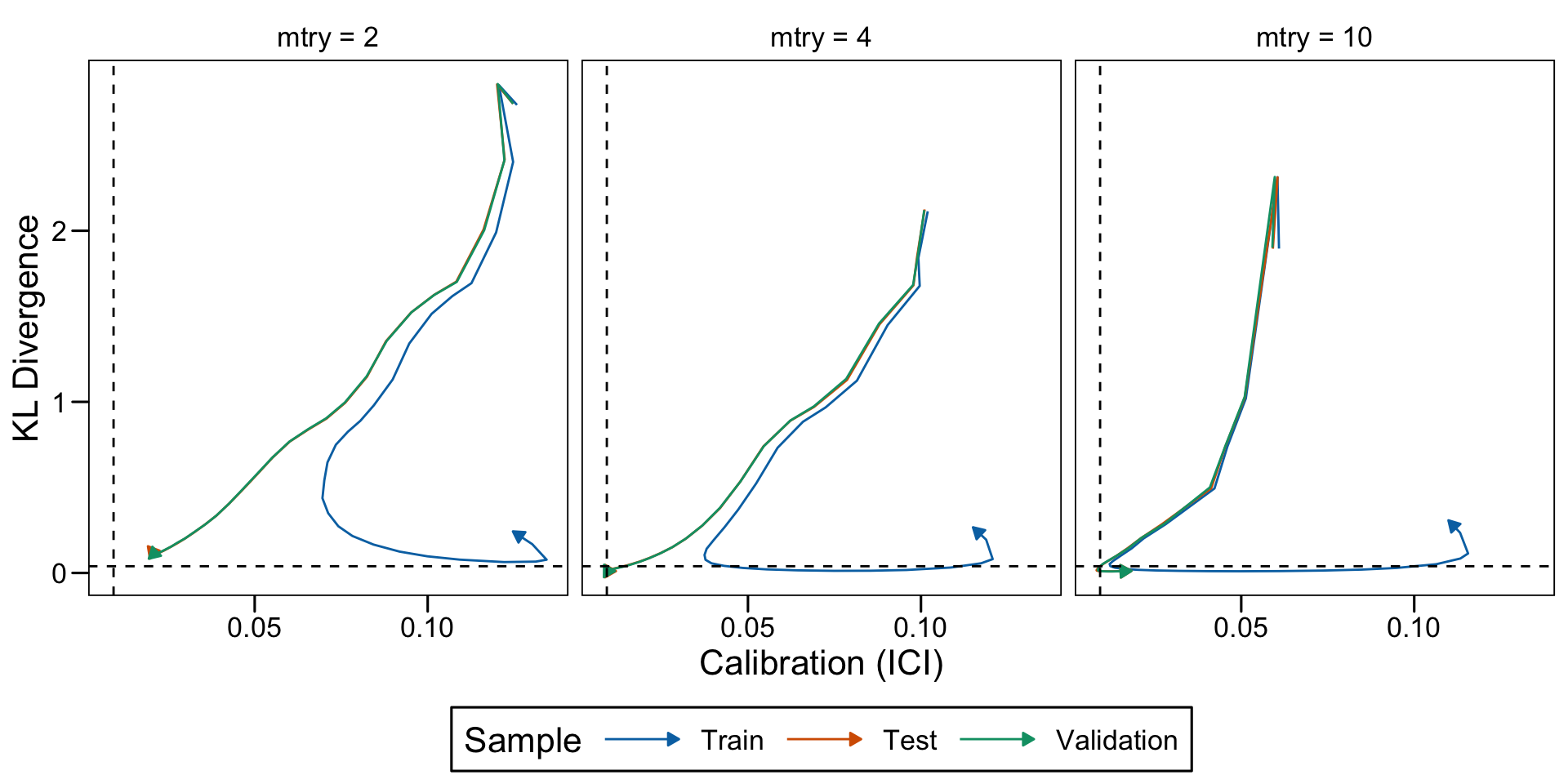
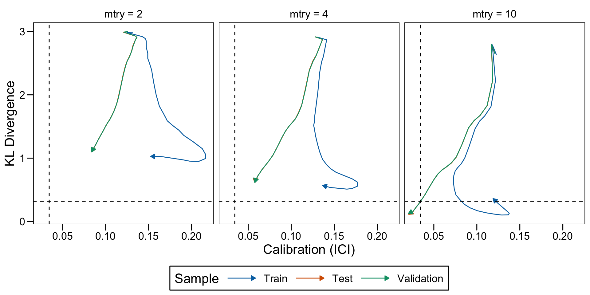
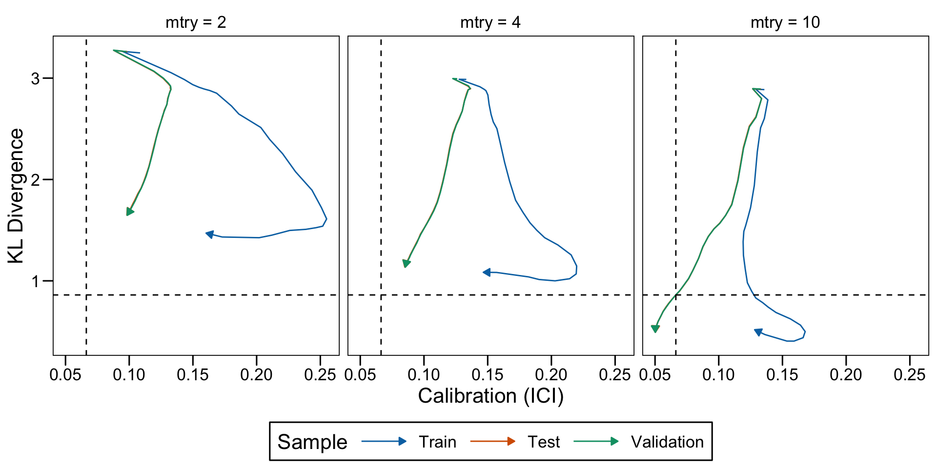
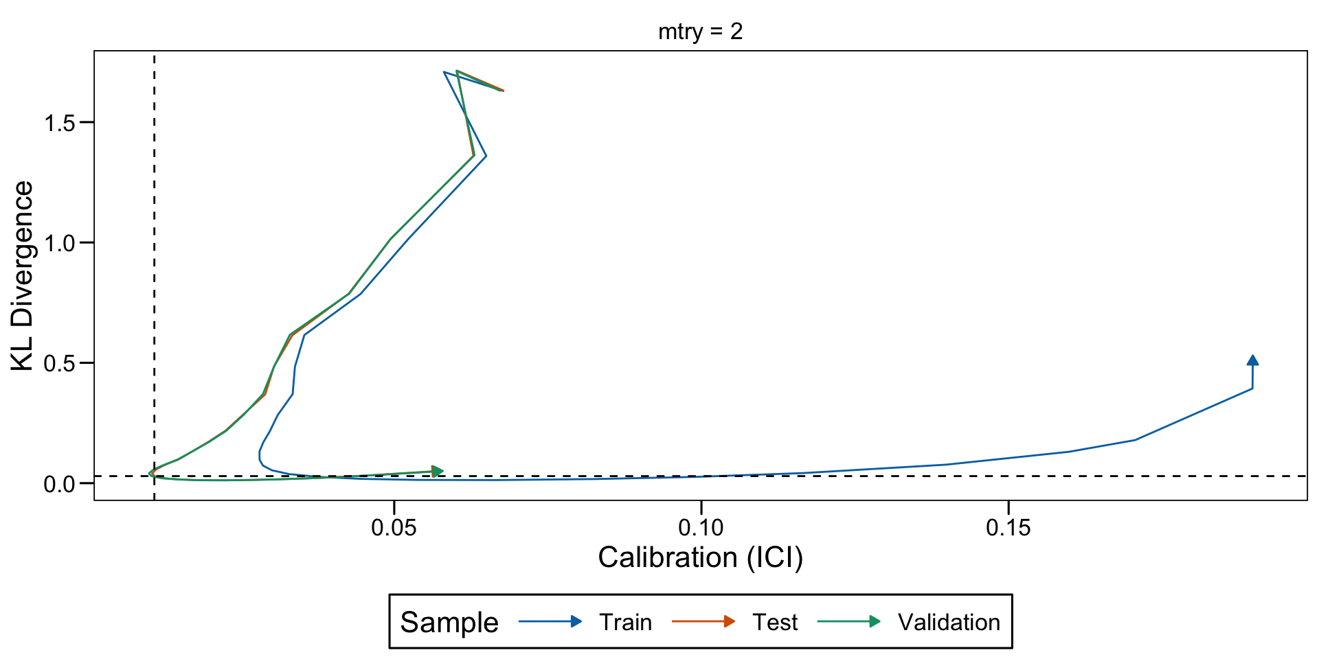
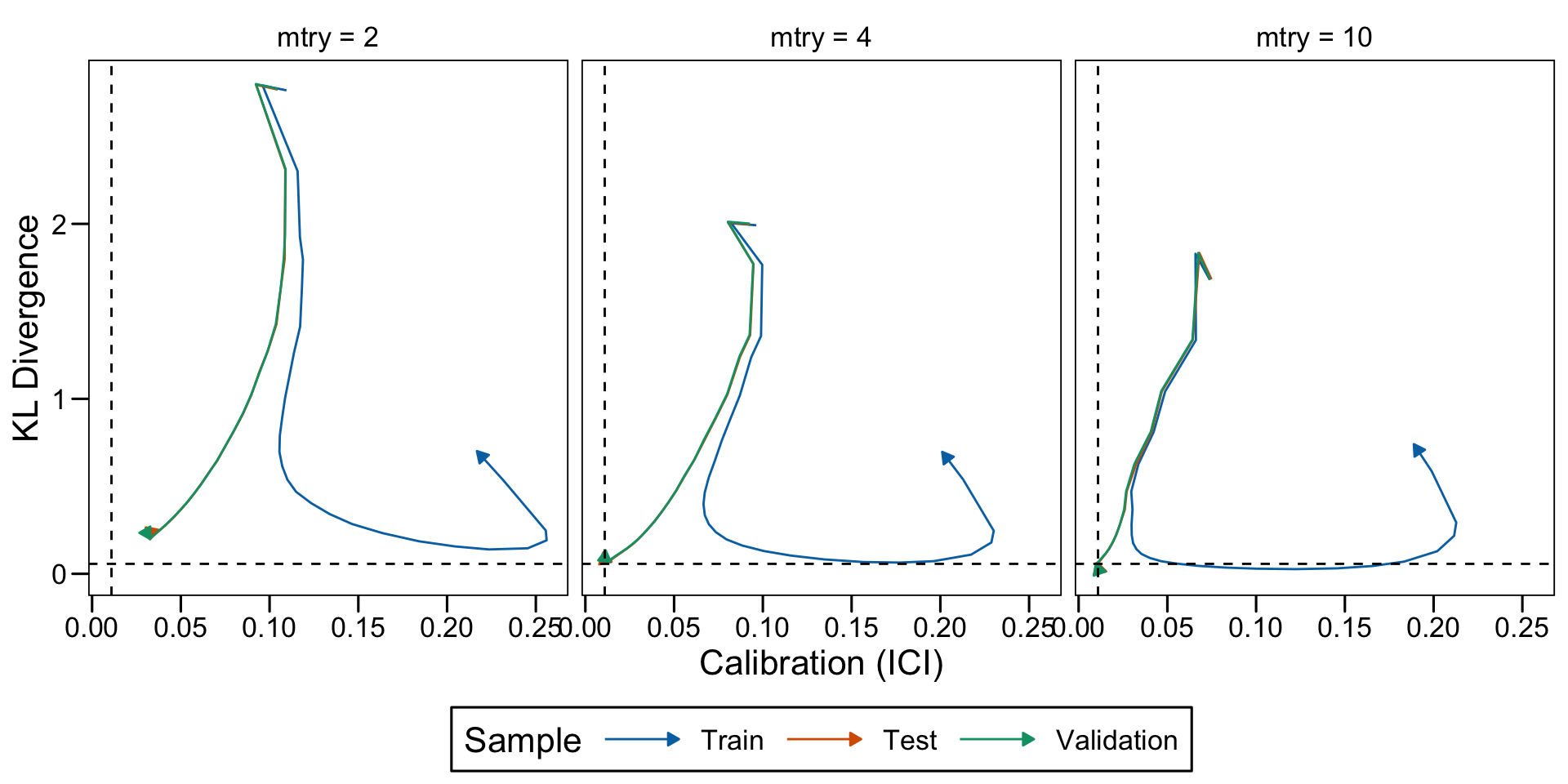
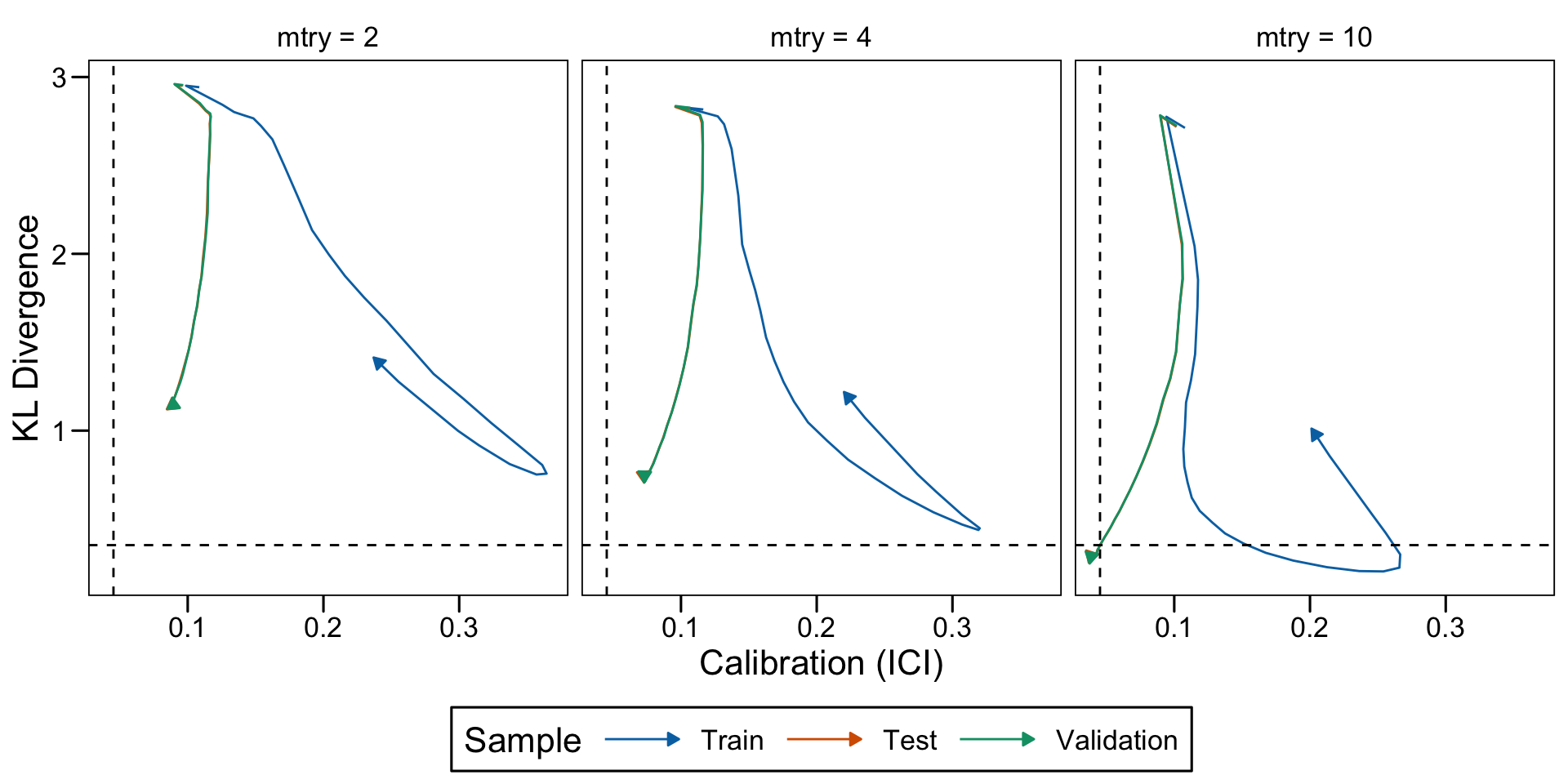
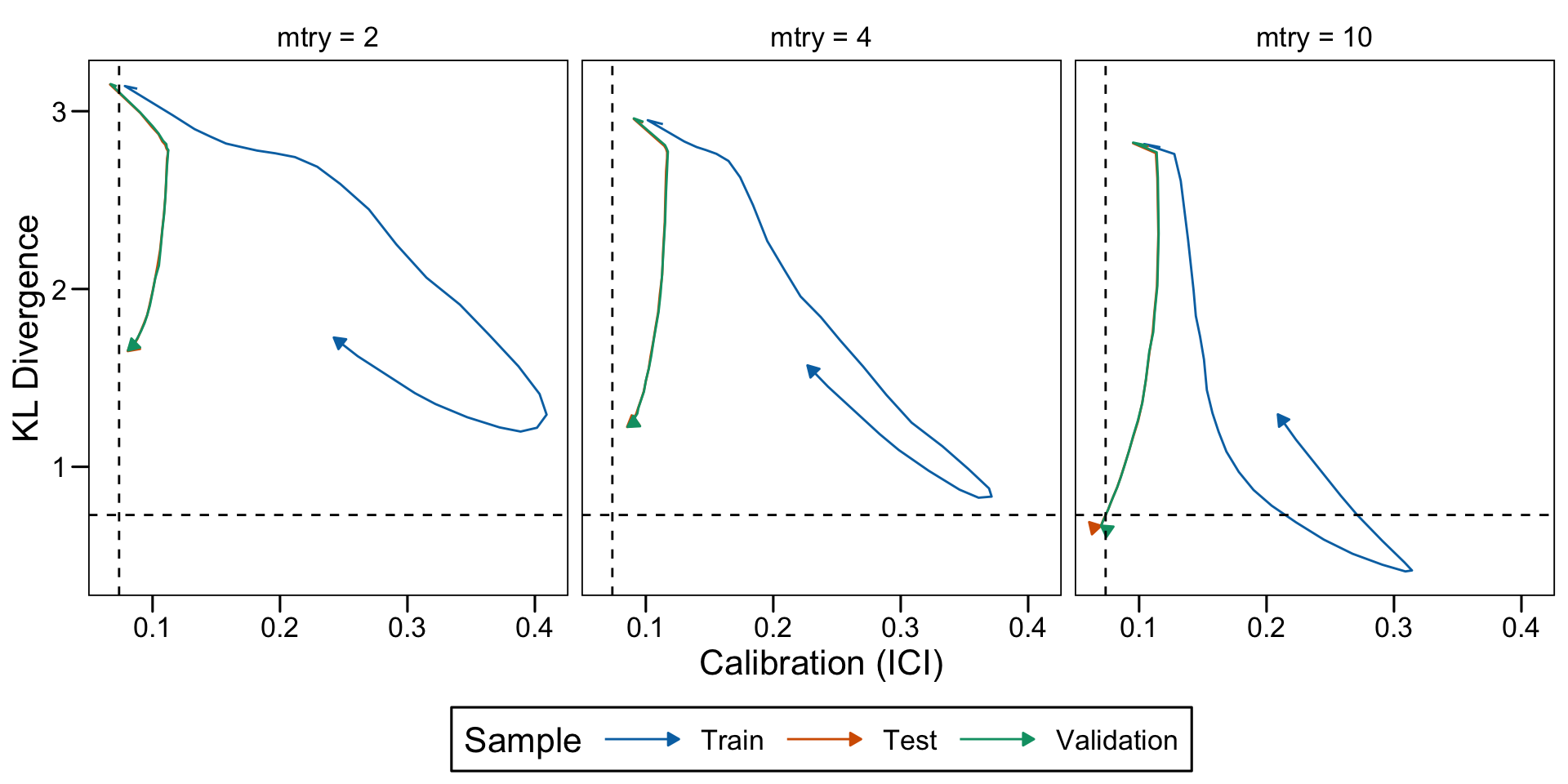
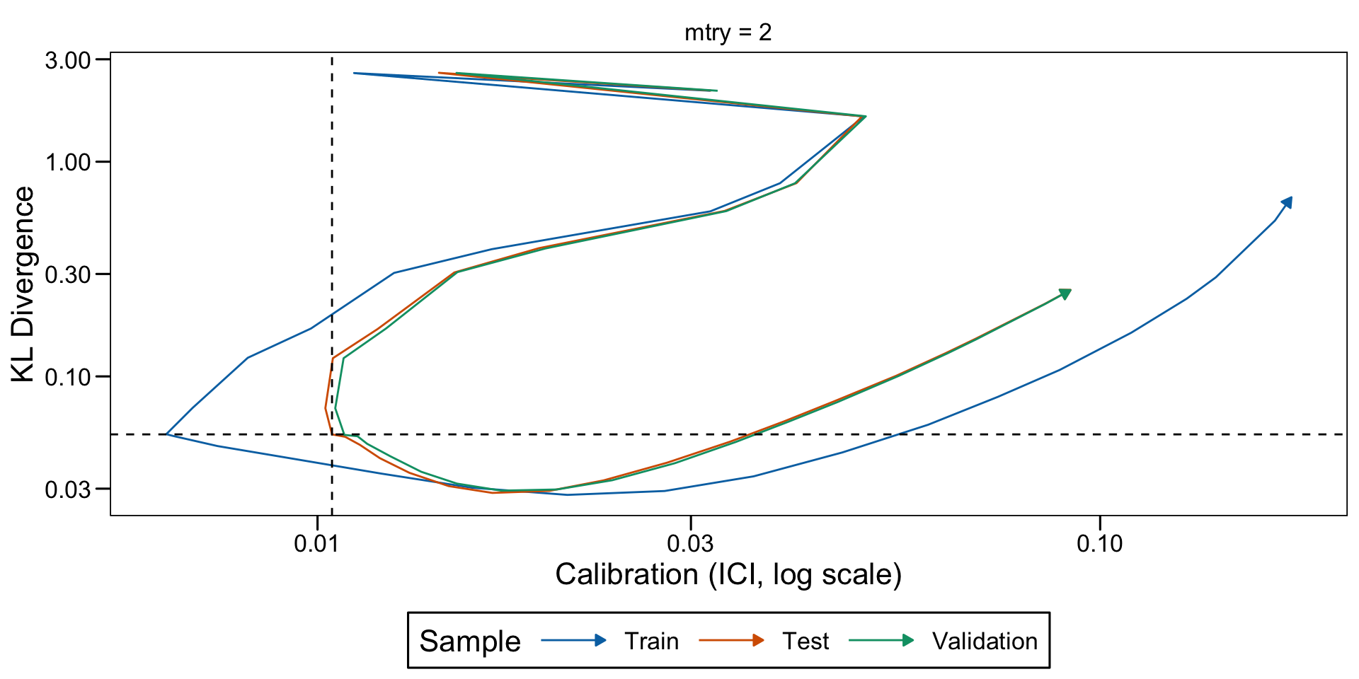
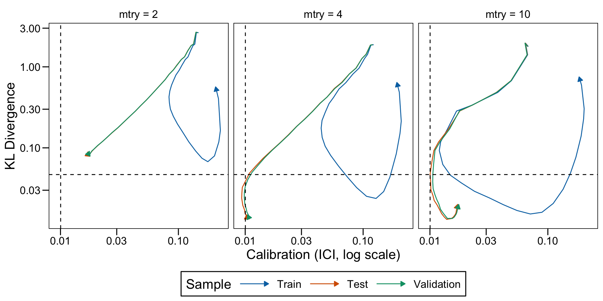
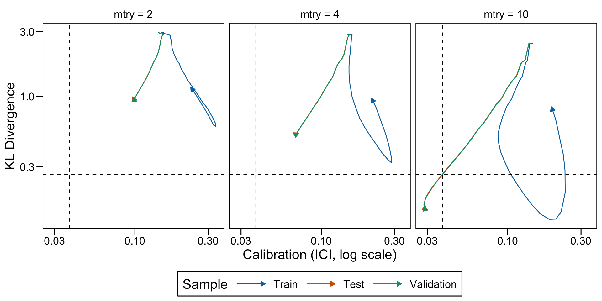
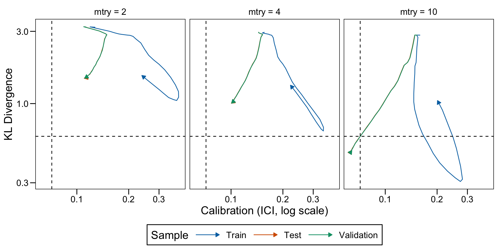
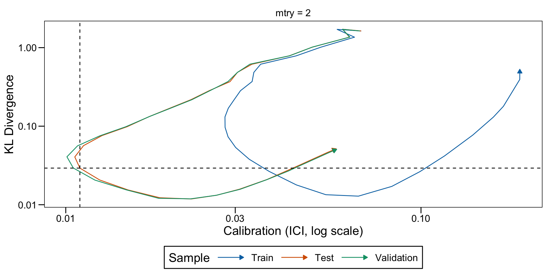
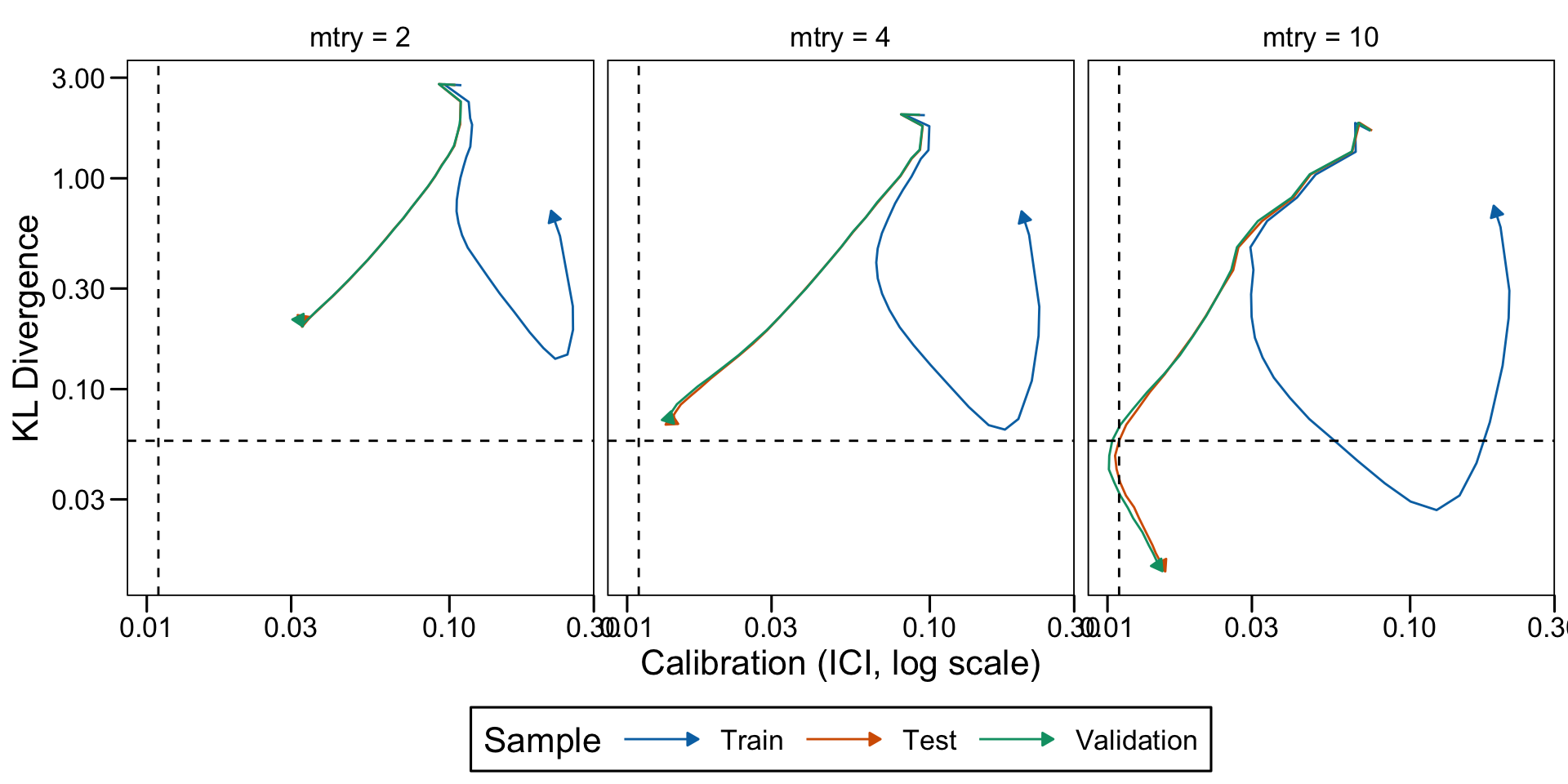
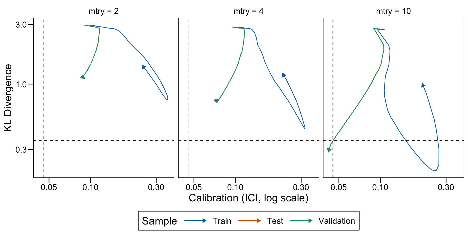
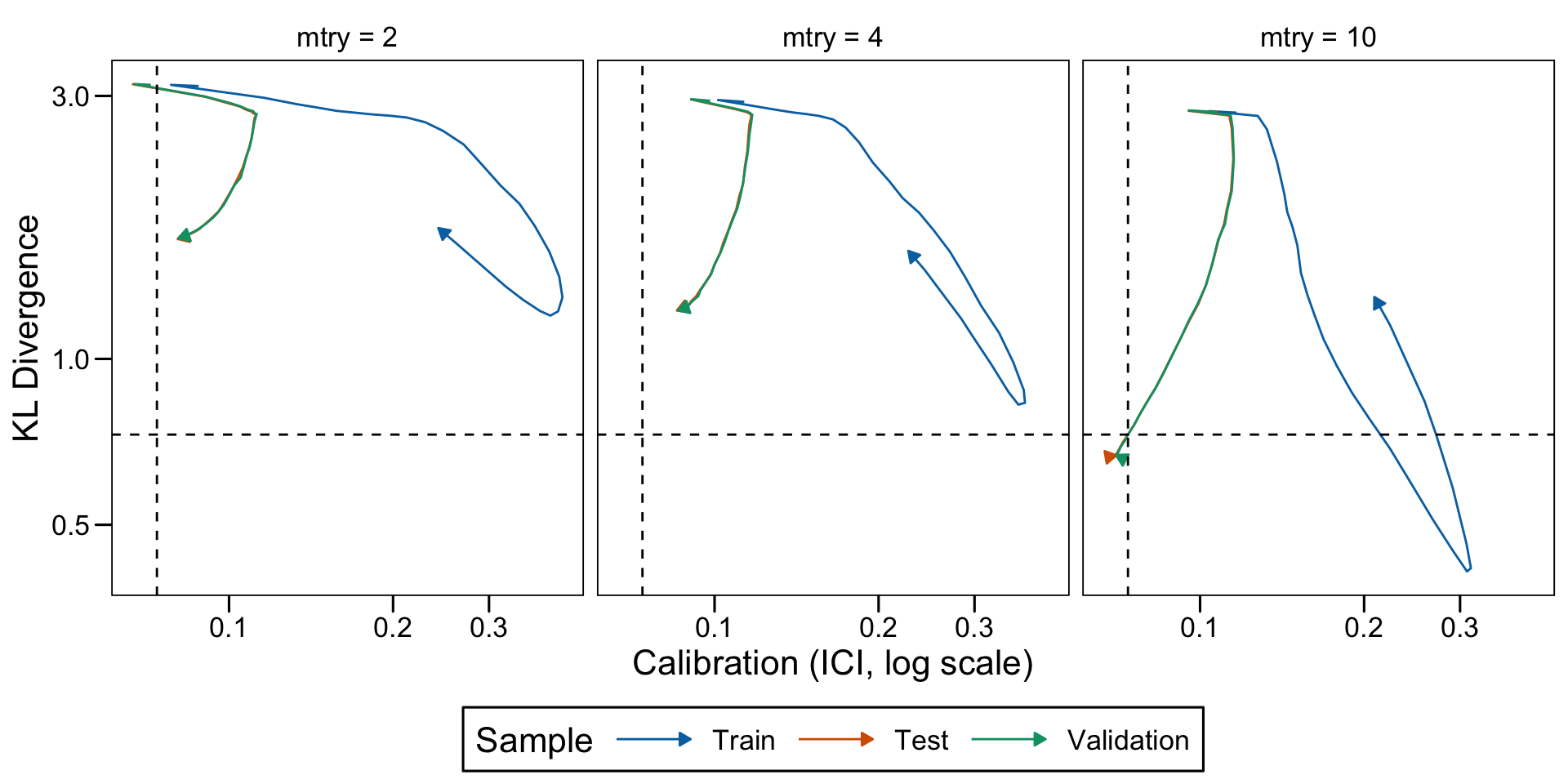
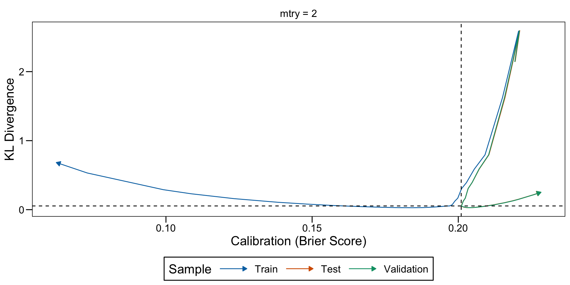
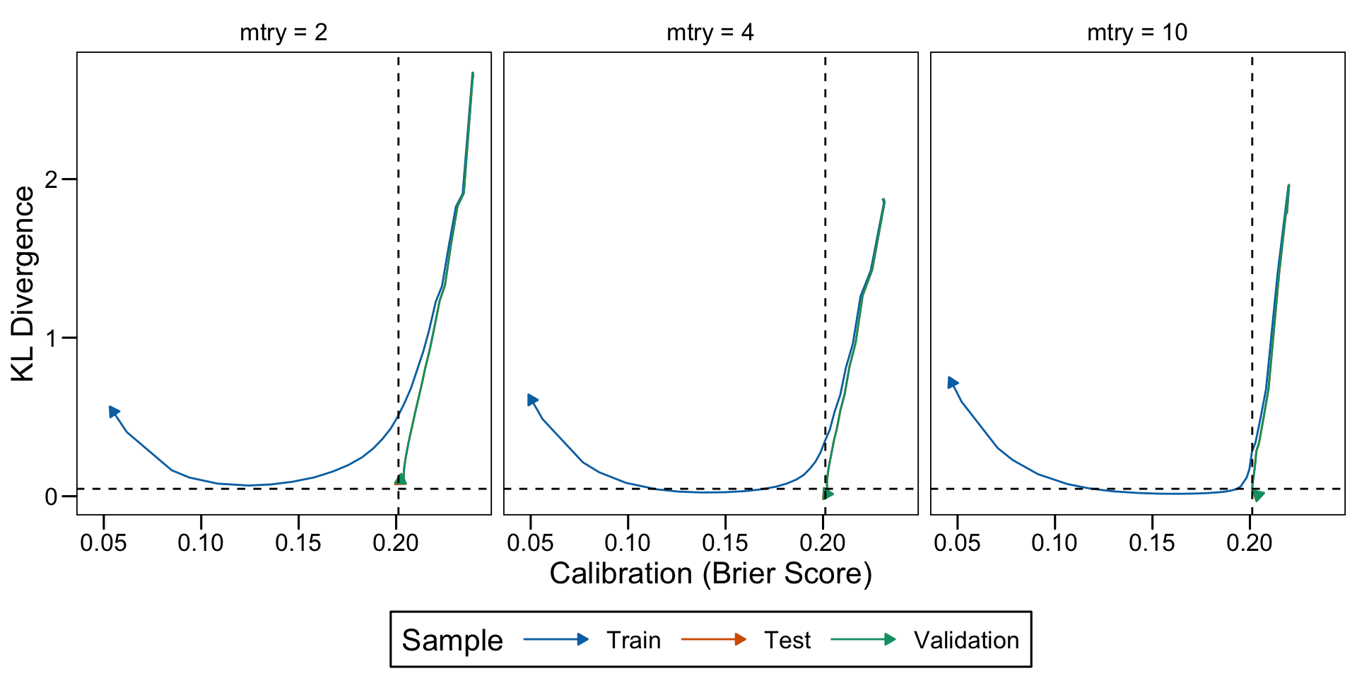
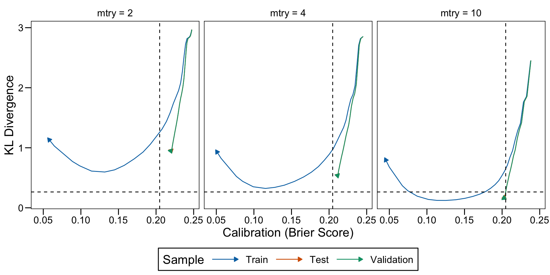
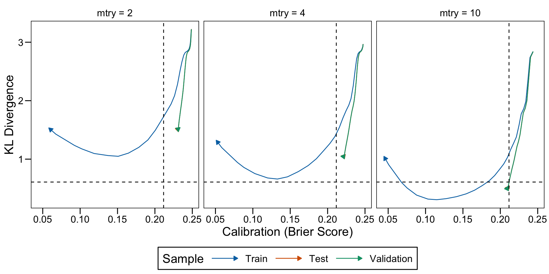
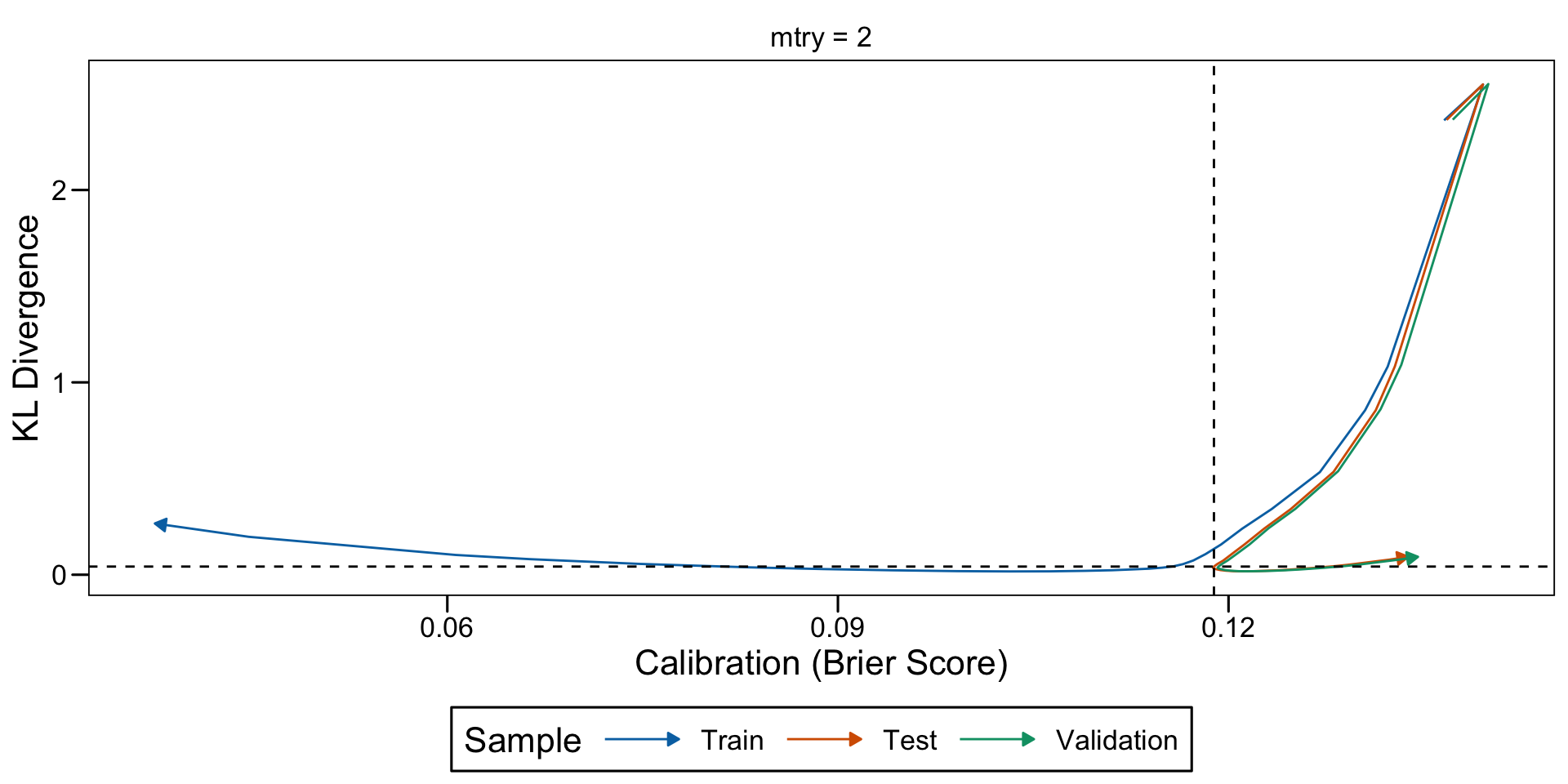
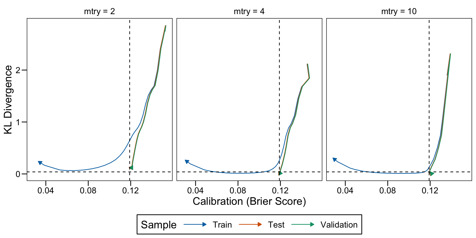
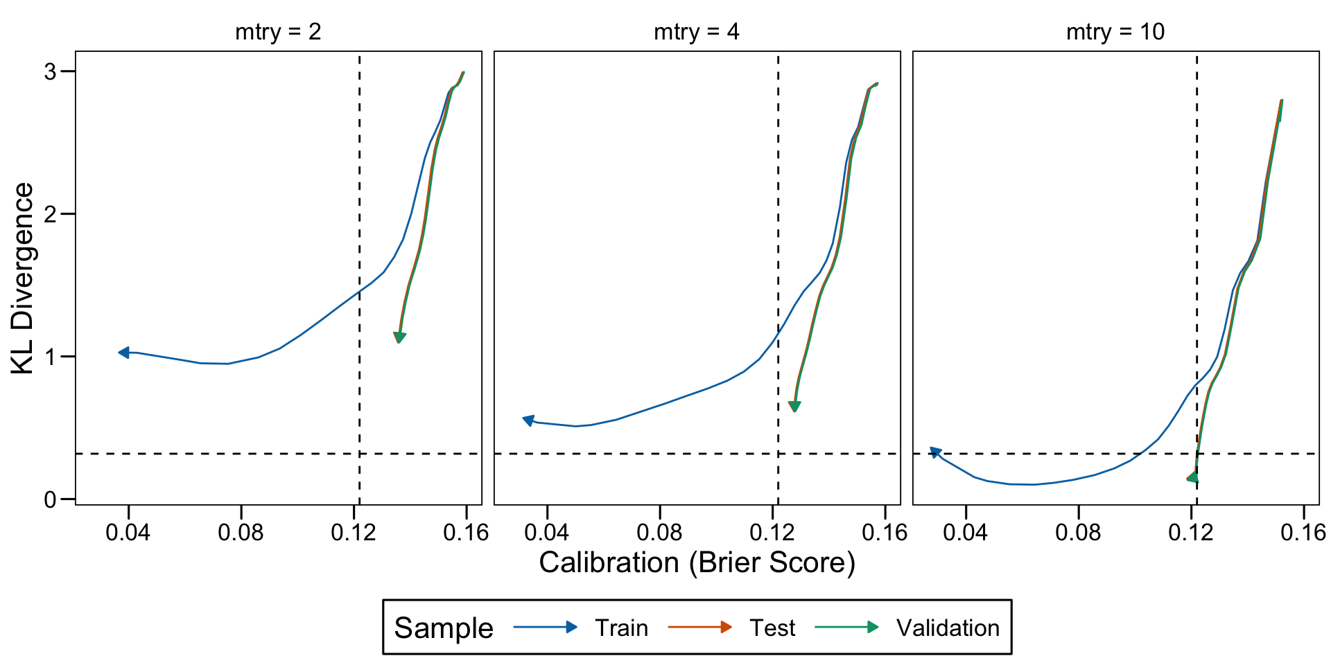
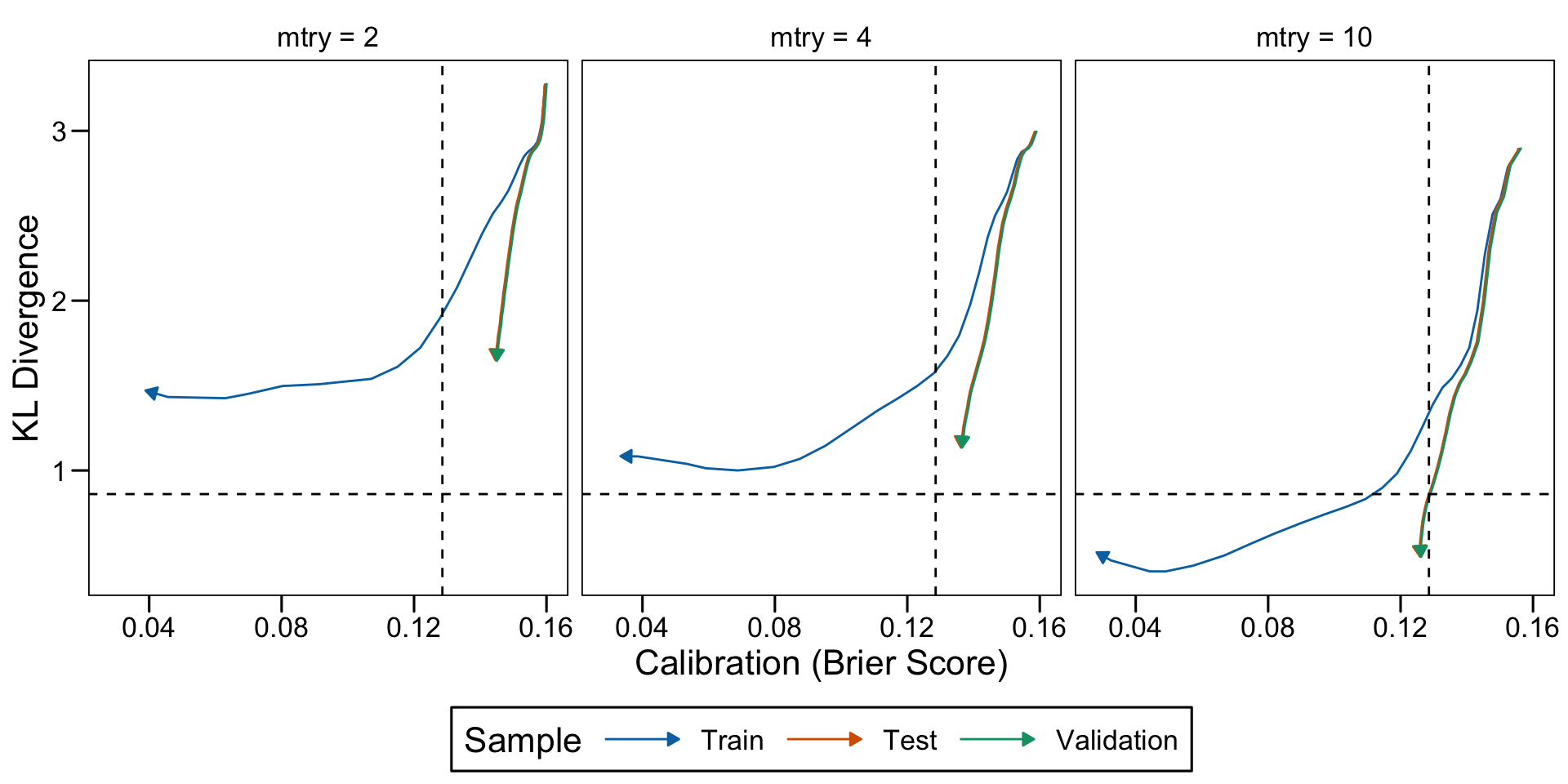
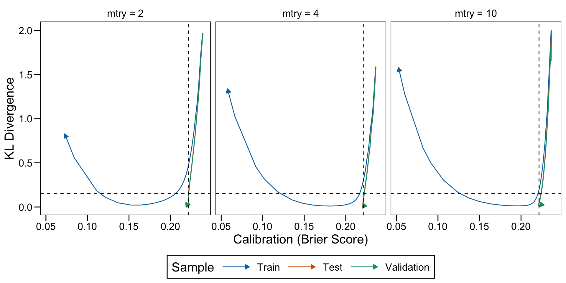
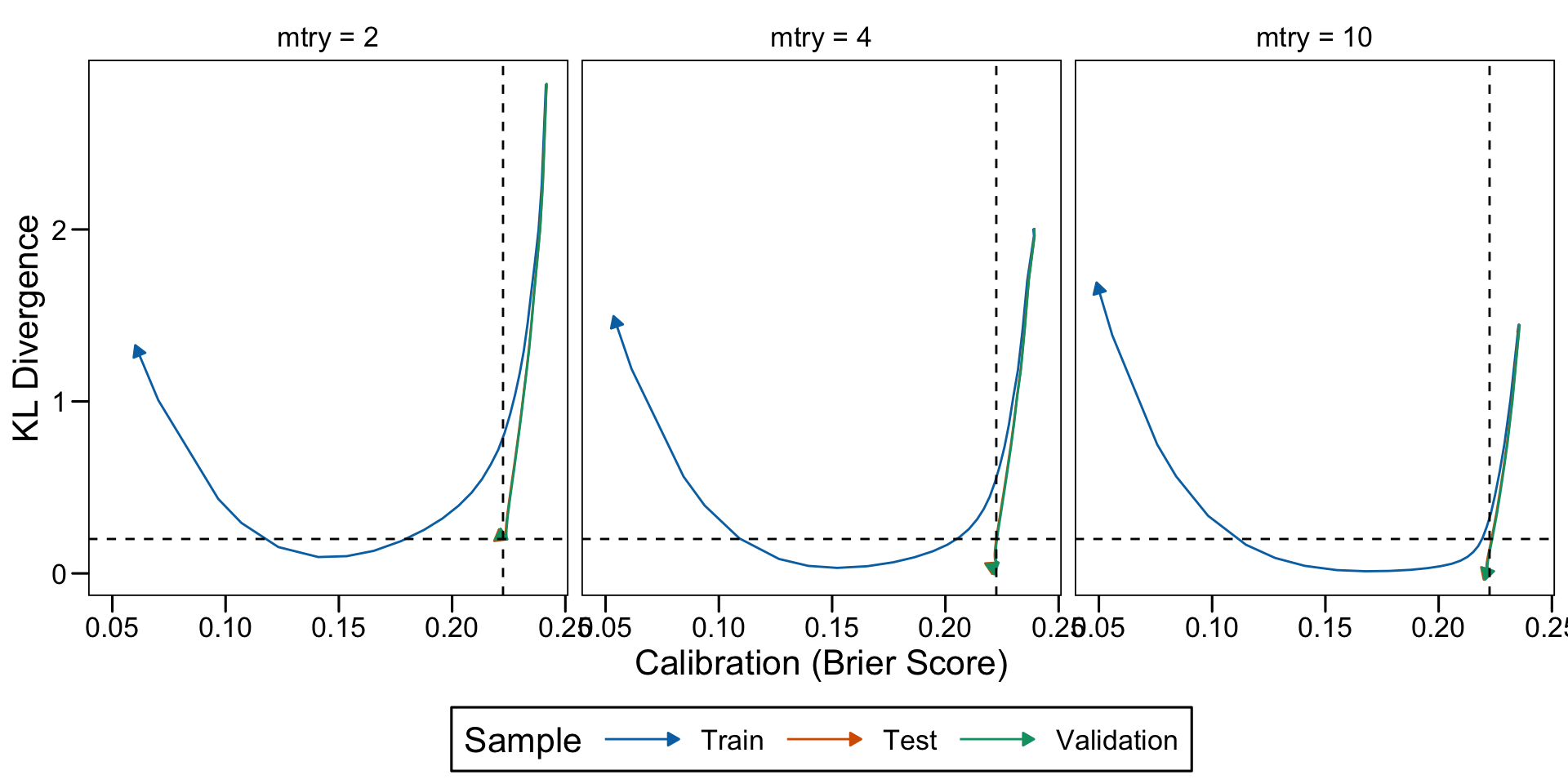
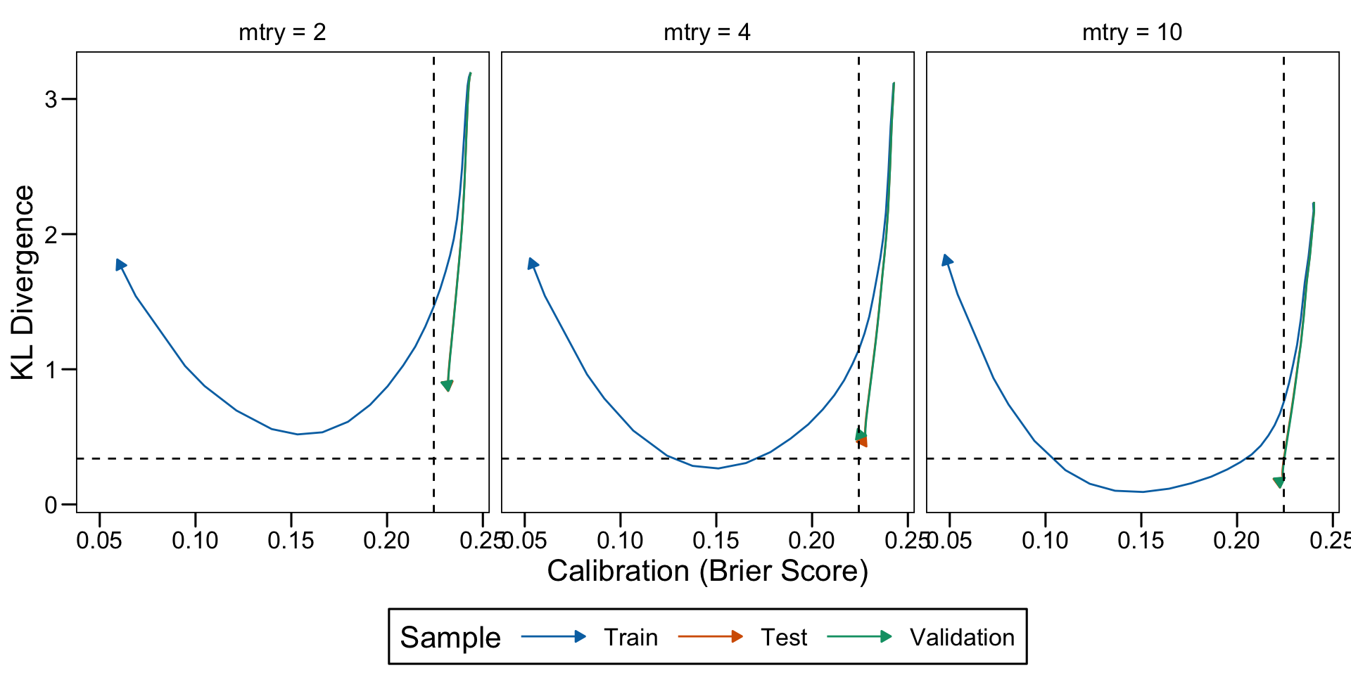
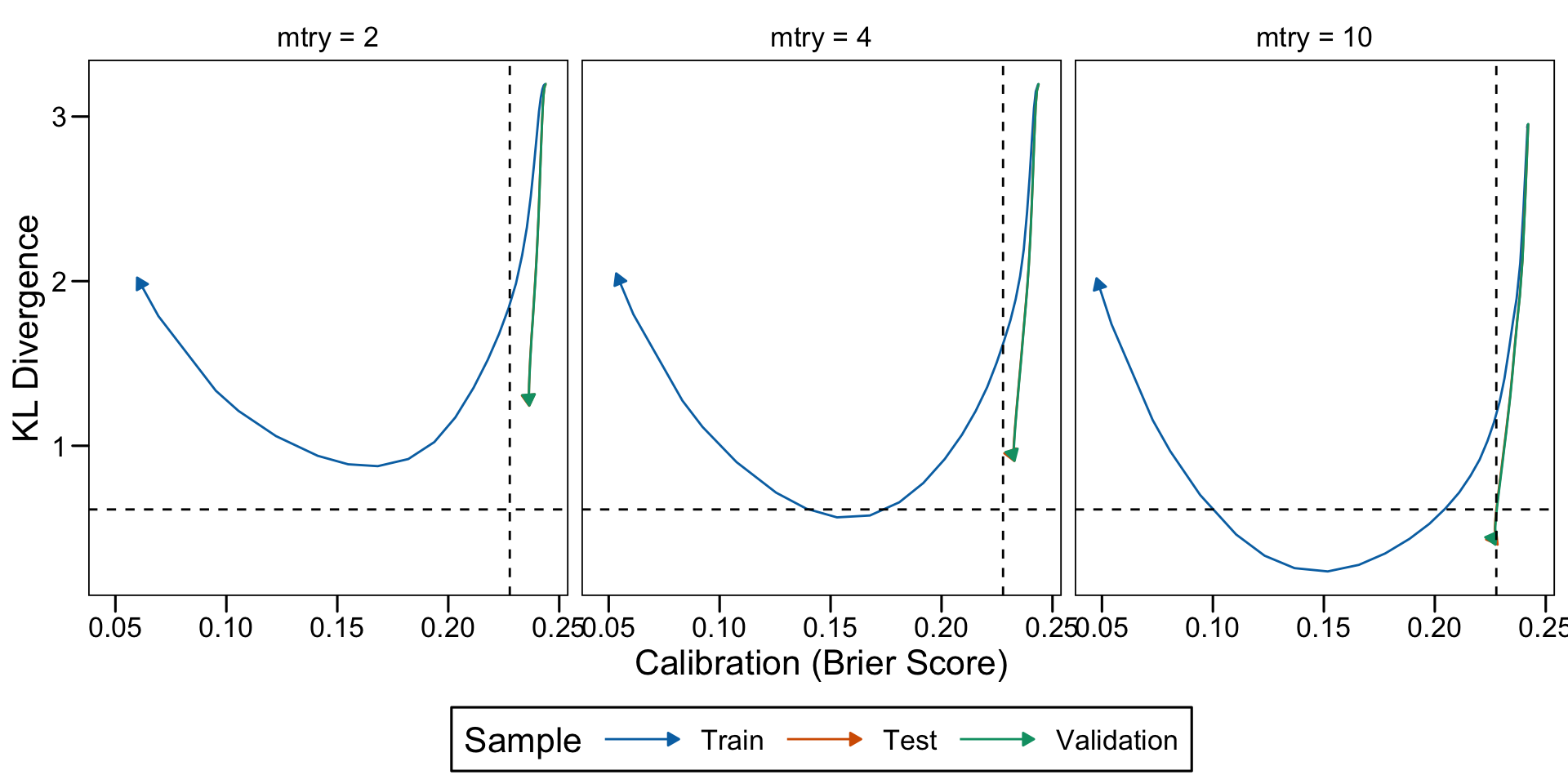
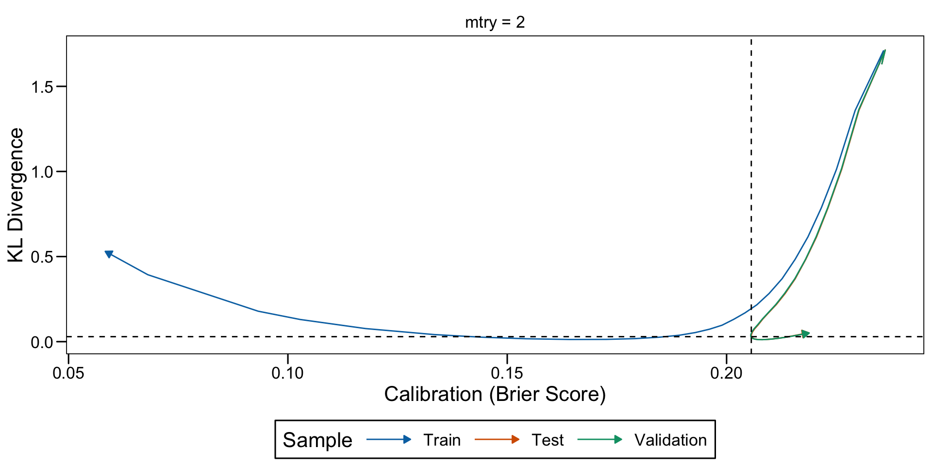
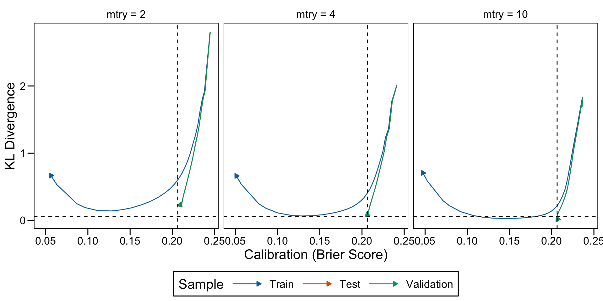
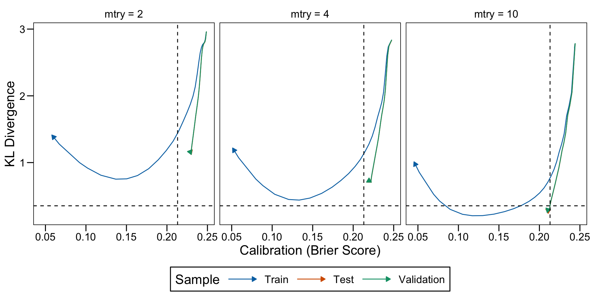
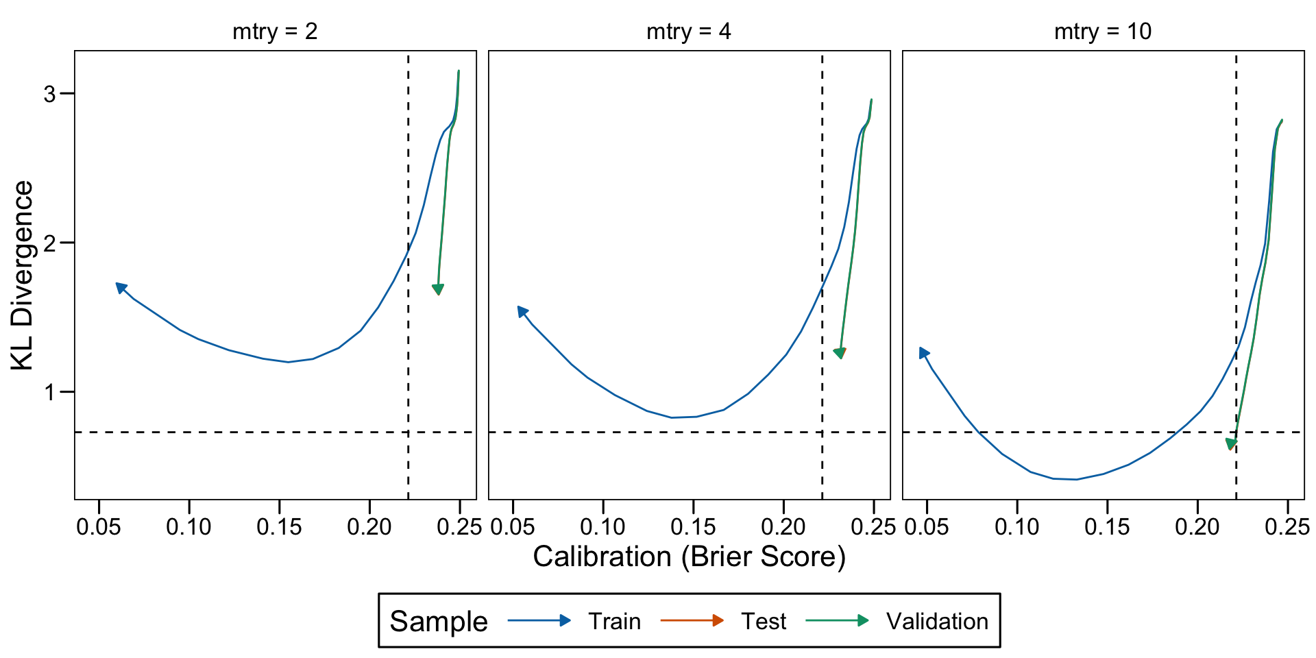
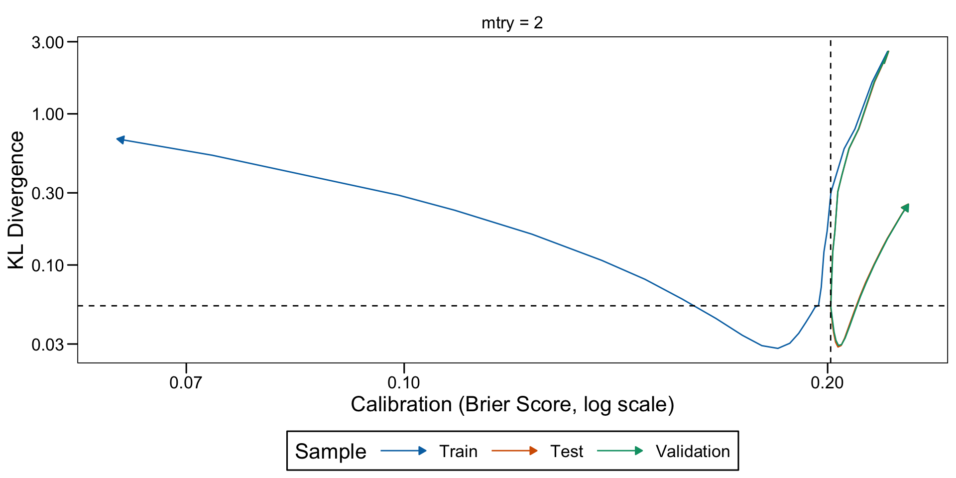
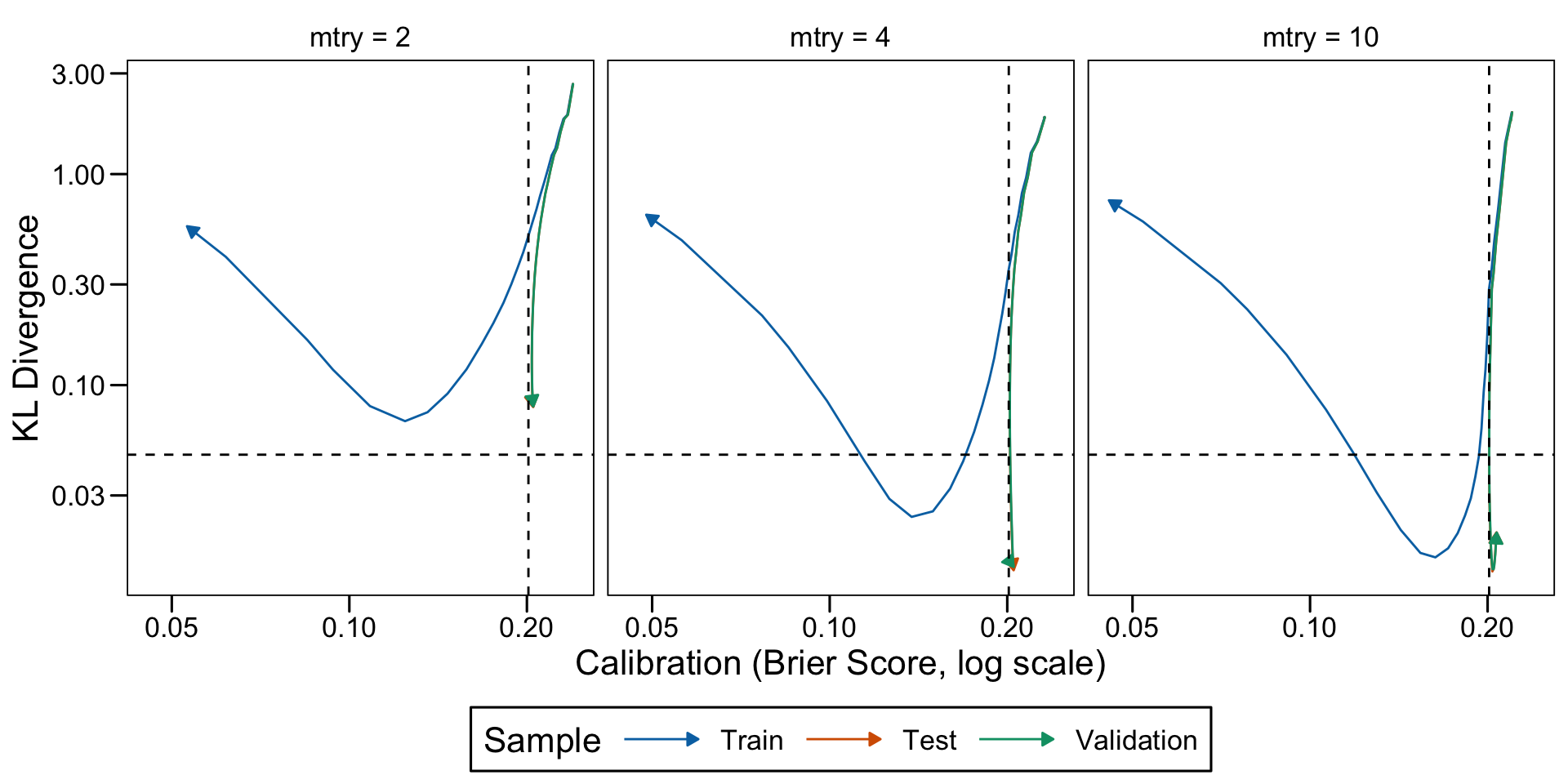
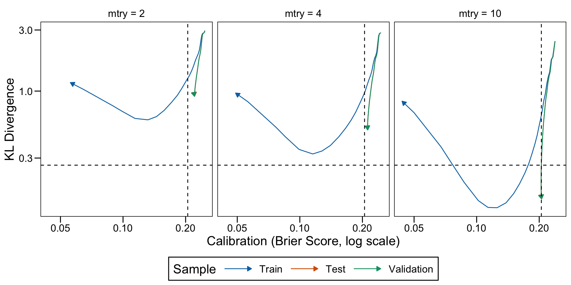
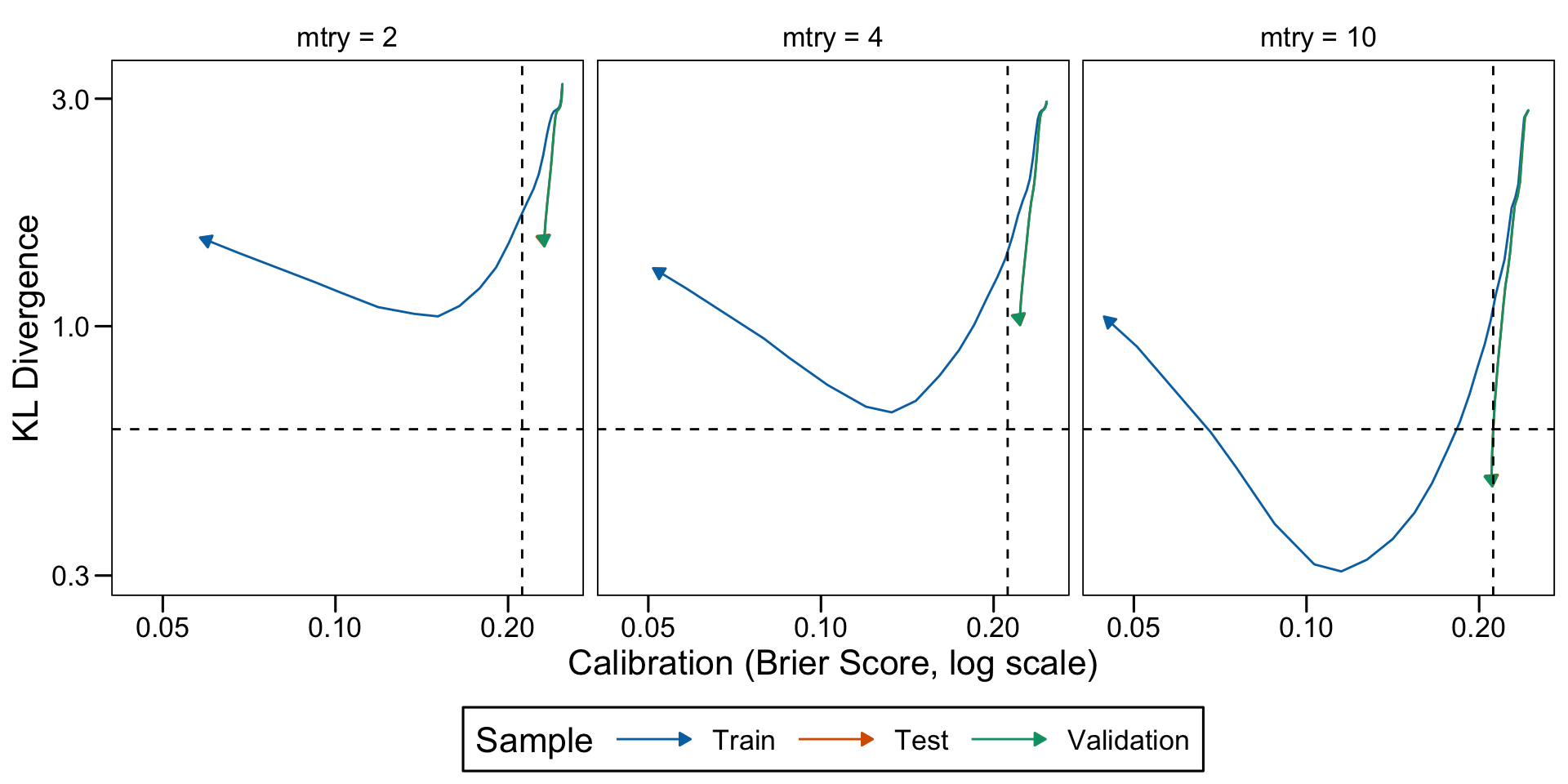
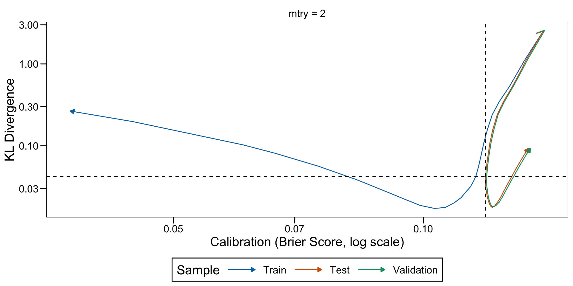
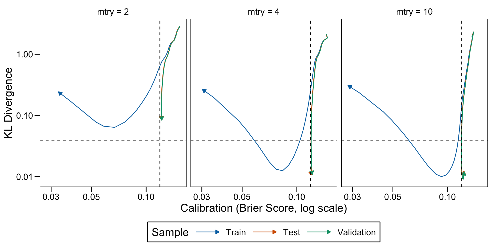
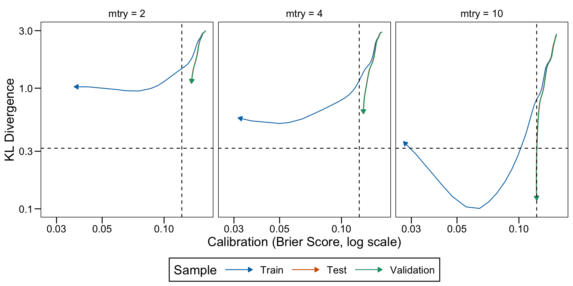
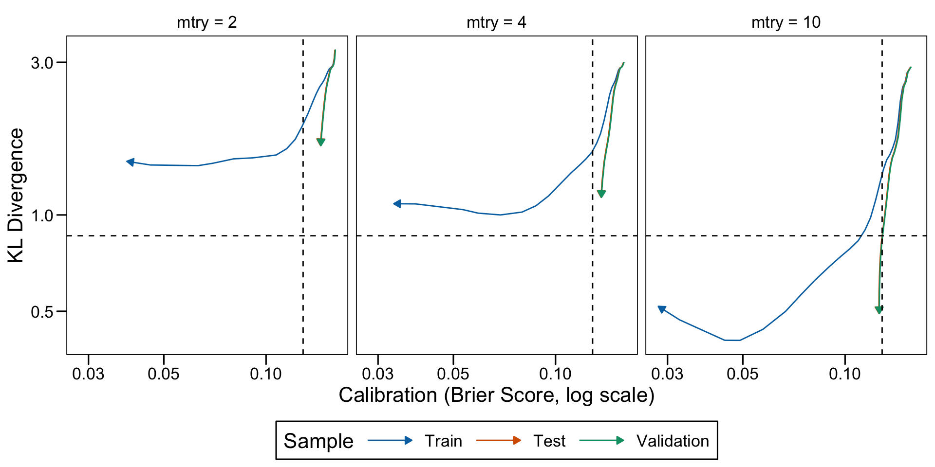
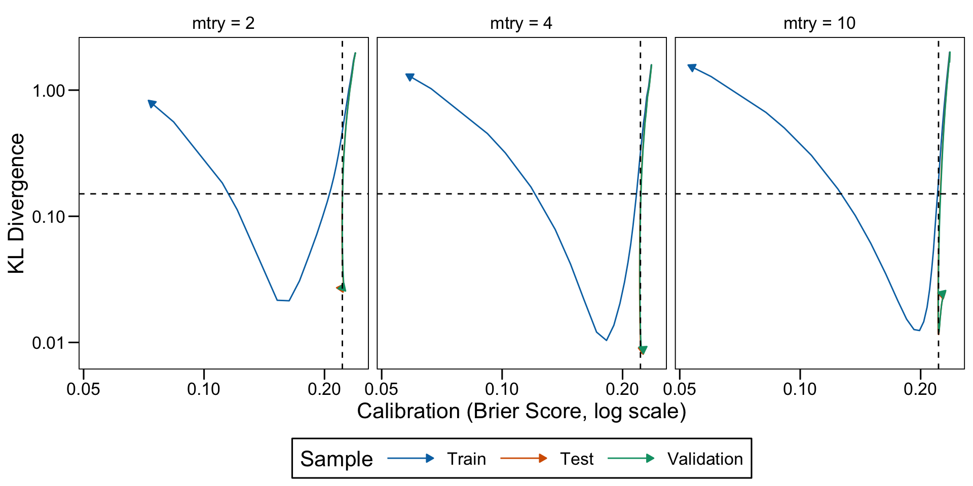
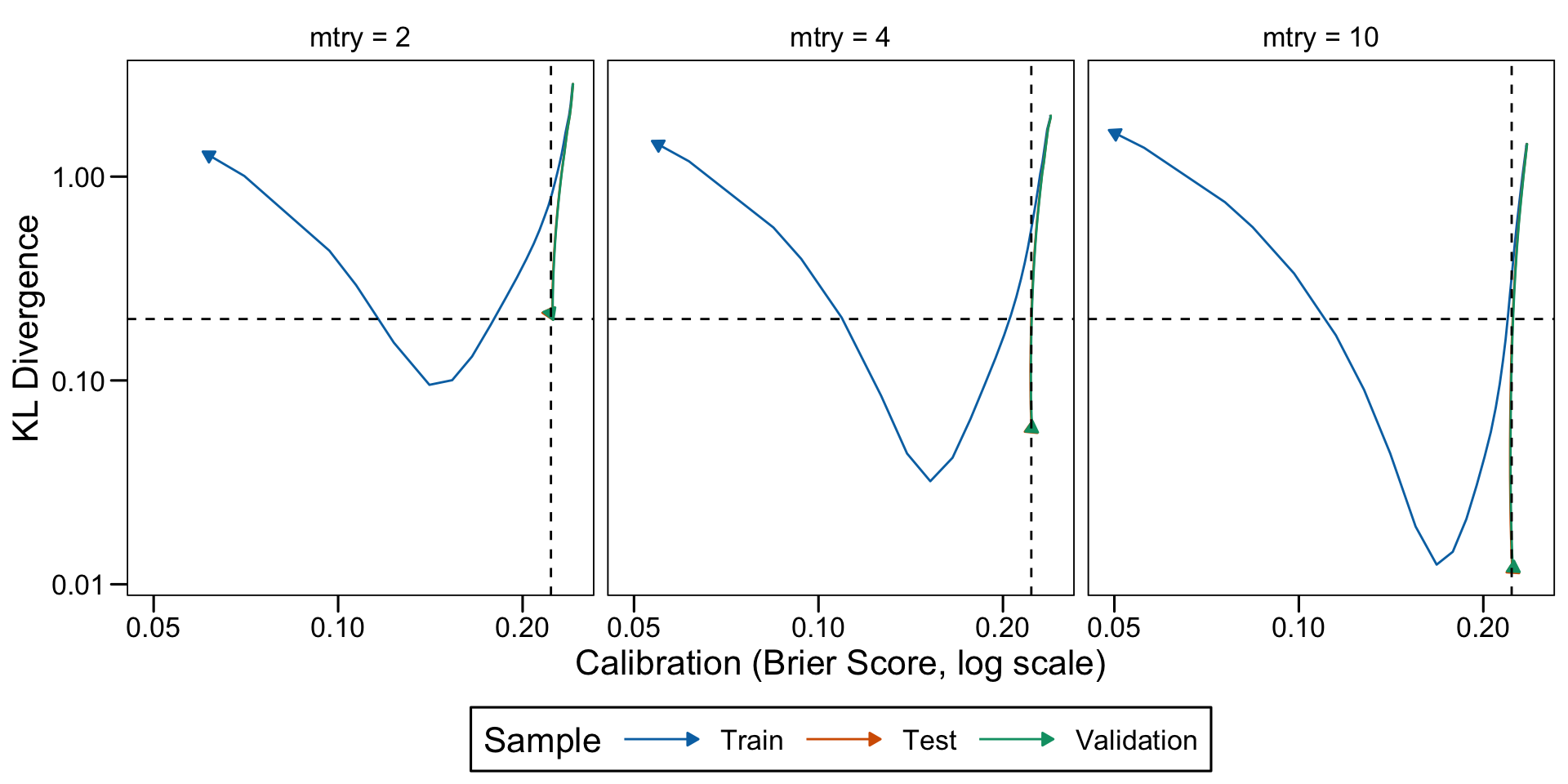
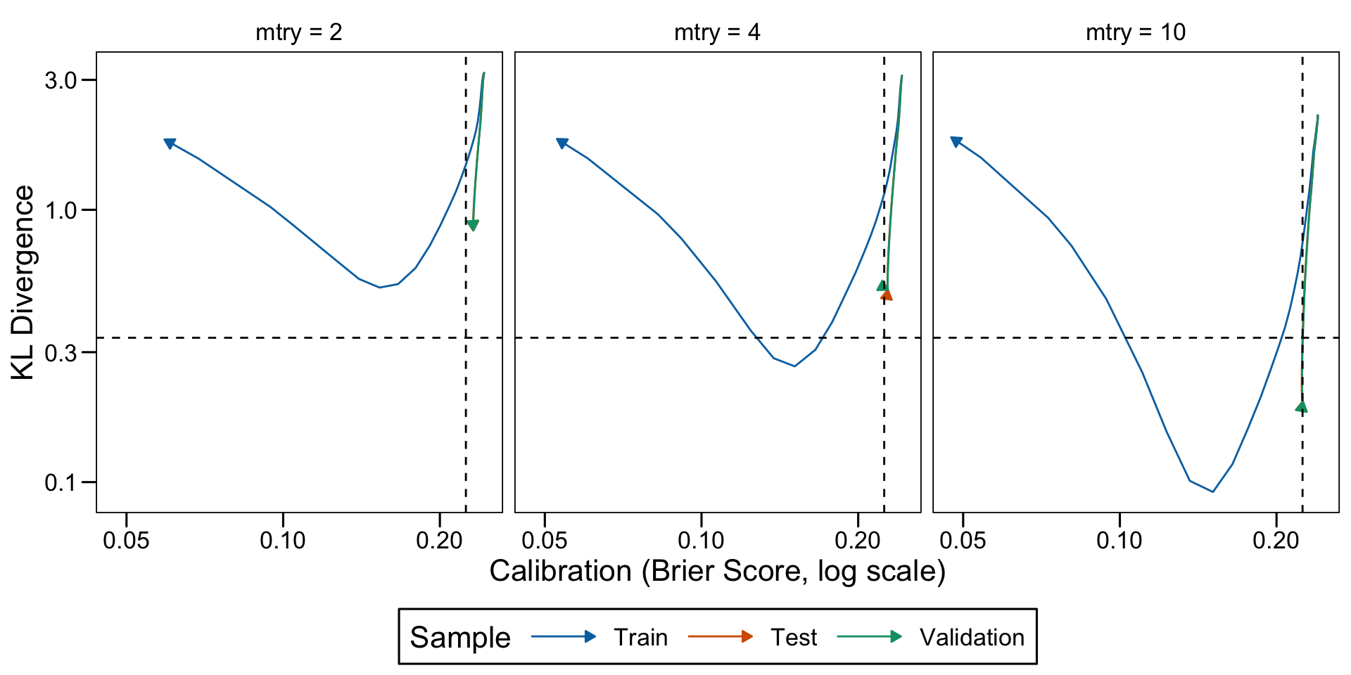
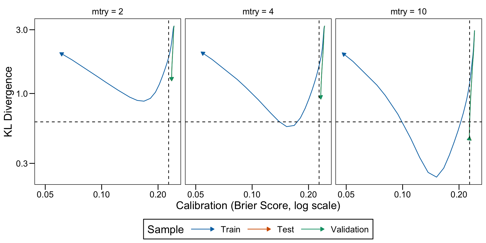
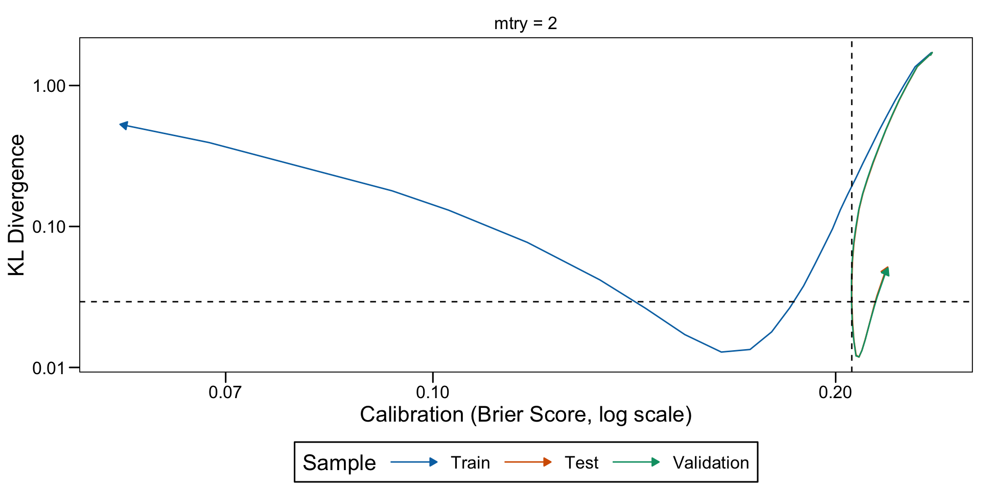
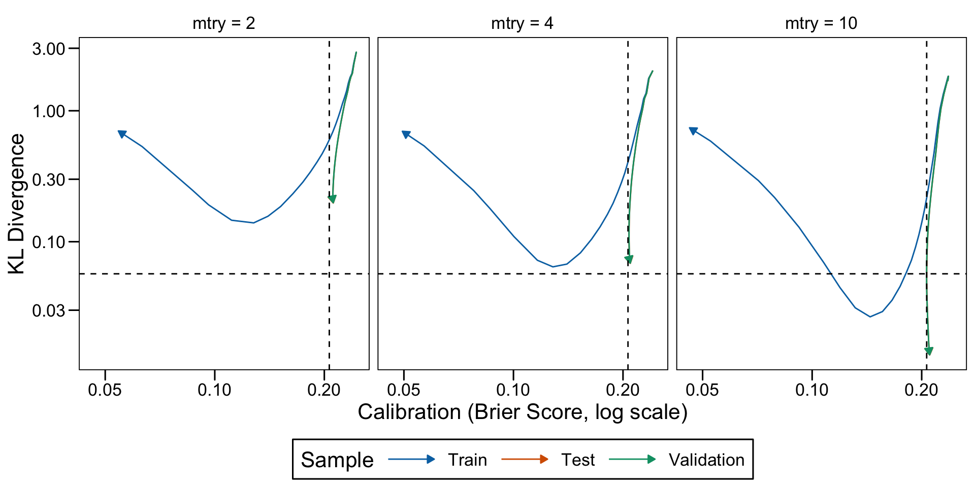
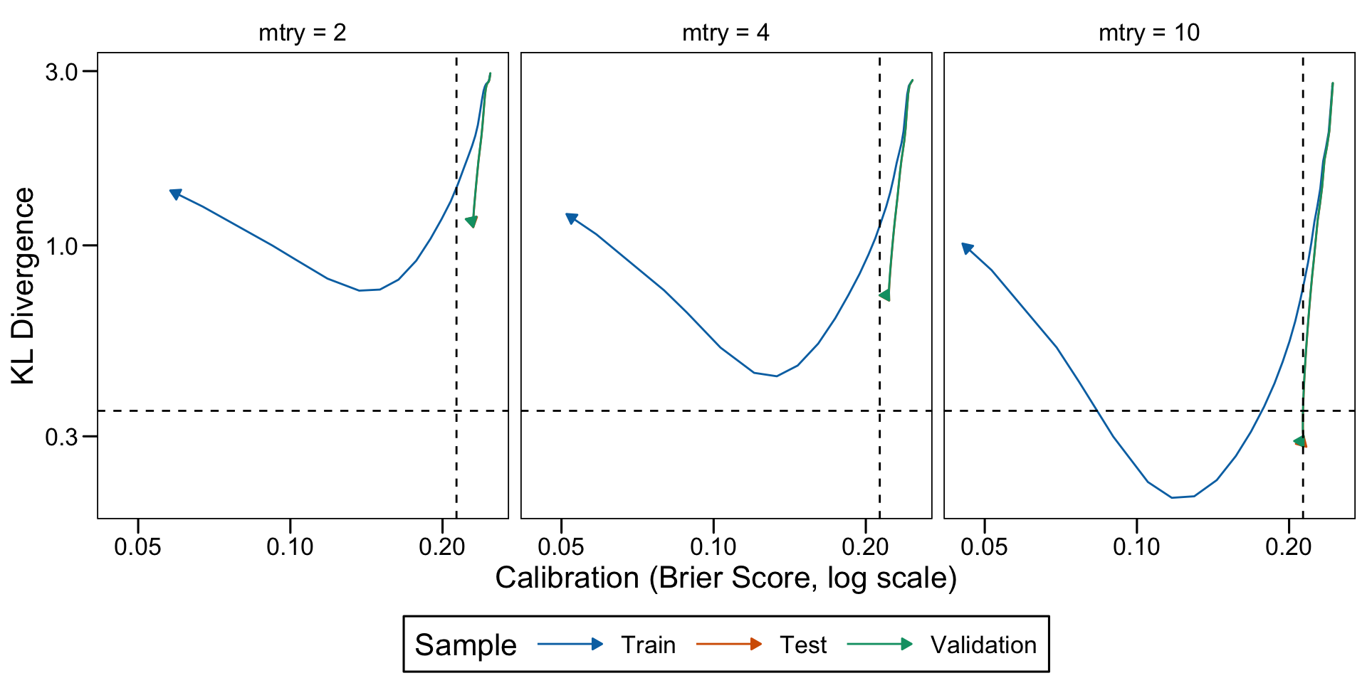
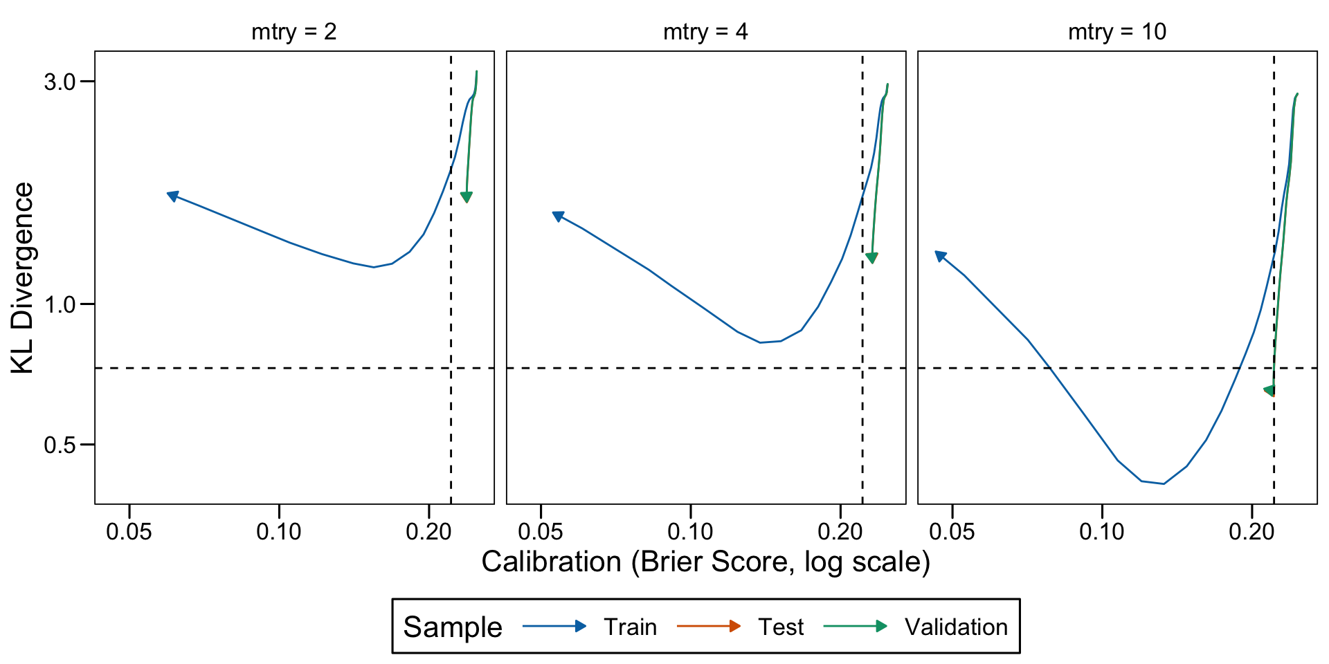
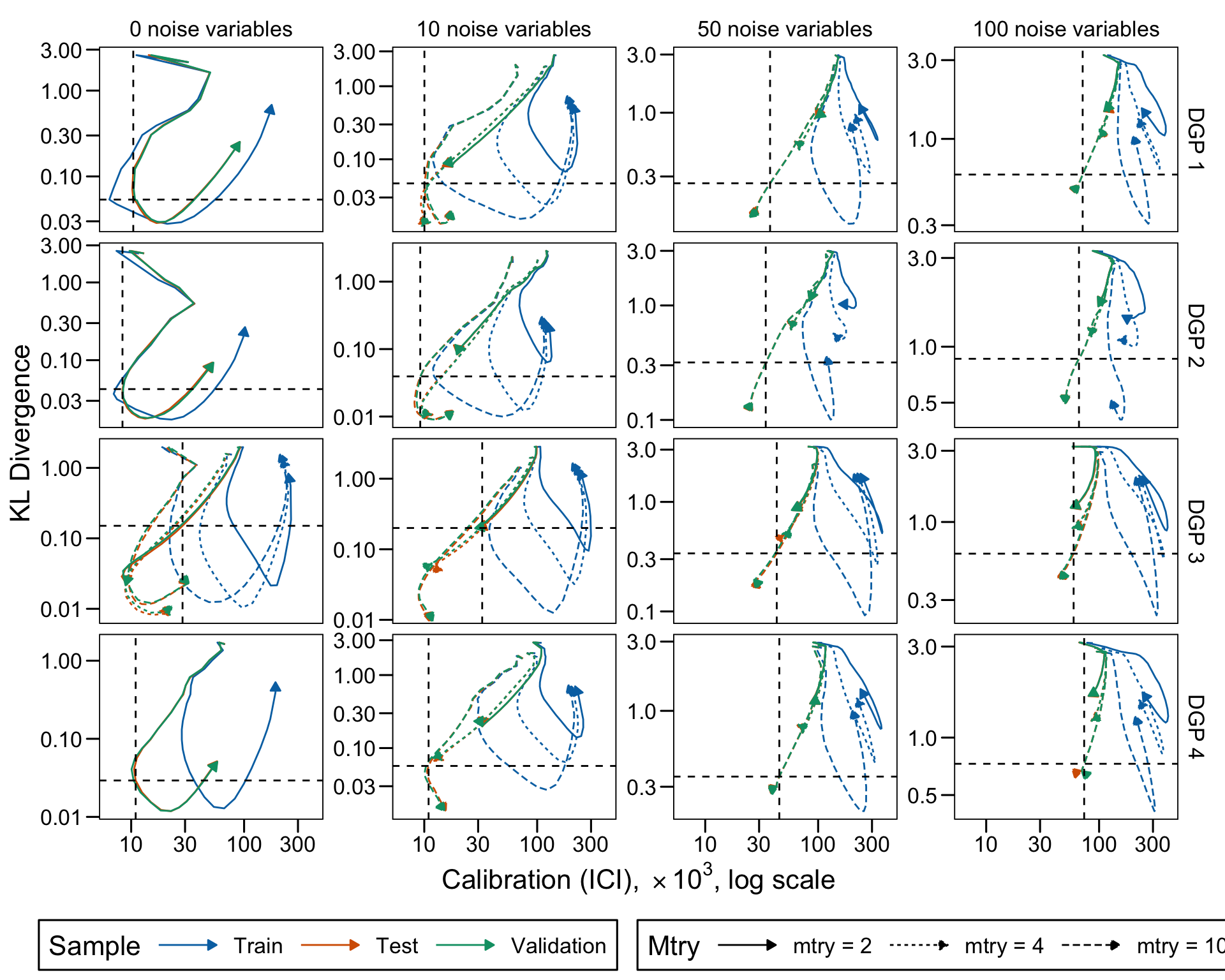
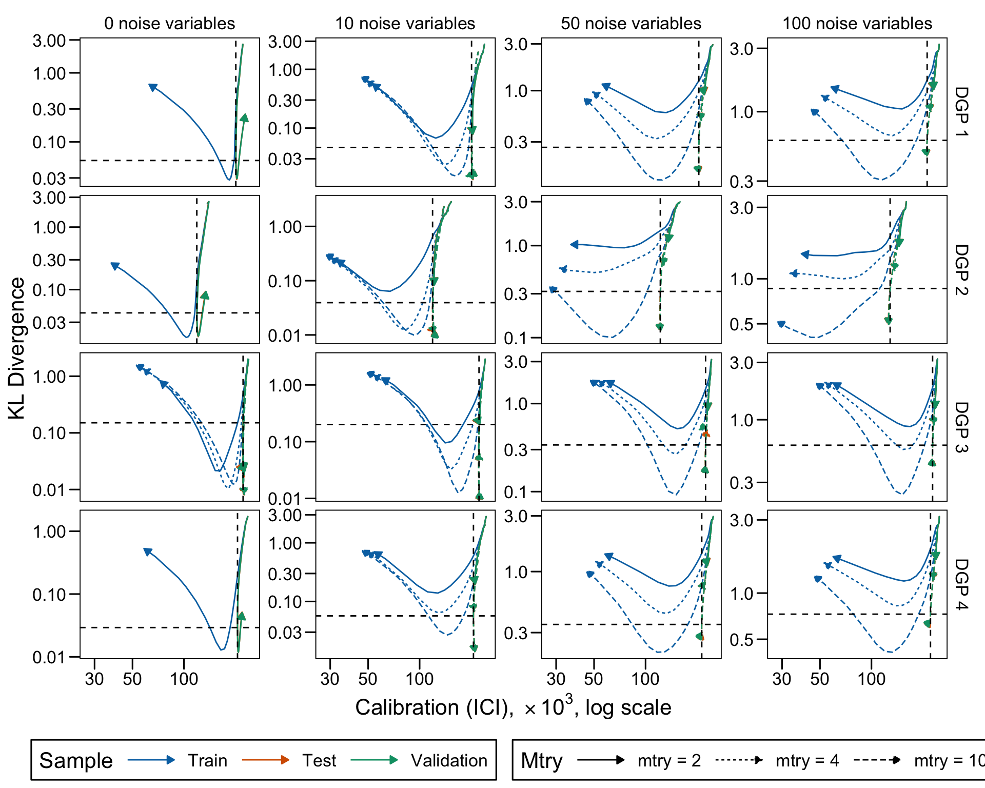
The dashed lines correspond to the values of the KL divergence and the calibration of the forest at which the AUC is the highest among the models of the grid search.

Complexity of a tree and relationship with calibration and divergence of scores to the true probabilities. (DGP 1, 0 noise variables)

Complexity of a tree and relationship with calibration and divergence of scores to the true probabilities. (DGP 1, 10 noise variables)

Complexity of a tree and relationship with calibration and divergence of scores to the true probabilities. (DGP 1, 50 noise variables)

Complexity of a tree and relationship with calibration and divergence of scores to the true probabilities. (DGP 1, 100 noise variables)

Complexity of a tree and relationship with calibration and divergence of scores to the true probabilities. (DGP 2, 0 noise variables)

Complexity of a tree and relationship with calibration and divergence of scores to the true probabilities. (DGP 2, 10 noise variables)

Complexity of a tree and relationship with calibration and divergence of scores to the true probabilities. (DGP 2, 50 noise variables)

Complexity of a tree and relationship with calibration and divergence of scores to the true probabilities. (DGP 2, 100 noise variables)

Complexity of a tree and relationship with calibration and divergence of scores to the true probabilities. (DGP 3, 0 noise variables)

Complexity of a tree and relationship with calibration and divergence of scores to the true probabilities. (DGP 3, 10 noise variables)

Complexity of a tree and relationship with calibration and divergence of scores to the true probabilities. (DGP 3, 50 noise variables)

Complexity of a tree and relationship with calibration and divergence of scores to the true probabilities. (DGP 3, 100 noise variables)

Complexity of a tree and relationship with calibration and divergence of scores to the true probabilities. (DGP 4, 0 noise variables)

Complexity of a tree and relationship with calibration and divergence of scores to the true probabilities. (DGP 4, 10 noise variables)

Complexity of a tree and relationship with calibration and divergence of scores to the true probabilities. (DGP 4, 50 noise variables)

Complexity of a tree and relationship with calibration and divergence of scores to the true probabilities. (DGP 4, 100 noise variables)

Complexity of a tree and relationship with calibration and divergence of scores to the true probabilities. (DGP 1, 0 noise variables, log scale)

Complexity of a tree and relationship with calibration and divergence of scores to the true probabilities. (DGP 1, 10 noise variables, log scale)

Complexity of a tree and relationship with calibration and divergence of scores to the true probabilities. (DGP 1, 50 noise variables, log scale)

Complexity of a tree and relationship with calibration and divergence of scores to the true probabilities. (DGP 1, 100 noise variables, log scale)

Complexity of a tree and relationship with calibration and divergence of scores to the true probabilities. (DGP 2, 0 noise variables, log scale)

Complexity of a tree and relationship with calibration and divergence of scores to the true probabilities. (DGP 2, 10 noise variables, log scale)

Complexity of a tree and relationship with calibration and divergence of scores to the true probabilities. (DGP 2, 50 noise variables, log scale)

Complexity of a tree and relationship with calibration and divergence of scores to the true probabilities. (DGP 2, 100 noise variables, log scale)

Complexity of a tree and relationship with calibration and divergence of scores to the true probabilities. (DGP 3, 0 noise variables, log scale)

Complexity of a tree and relationship with calibration and divergence of scores to the true probabilities. (DGP 3, 10 noise variables, log scale)

Complexity of a tree and relationship with calibration and divergence of scores to the true probabilities. (DGP 3, 50 noise variables, log scale)

Complexity of a tree and relationship with calibration and divergence of scores to the true probabilities. (DGP 3, 100 noise variables, log scale)

Complexity of a tree and relationship with calibration and divergence of scores to the true probabilities. (DGP 4, 0 noise variables, log scale)

Complexity of a tree and relationship with calibration and divergence of scores to the true probabilities. (DGP 4, 10 noise variables, log scale)

Complexity of a tree and relationship with calibration and divergence of scores to the true probabilities. (DGP 4, 50 noise variables, log scale)

Complexity of a tree and relationship with calibration and divergence of scores to the true probabilities. (DGP 4, 100 noise variables, log scale)

We can also put all the scenarios in a single graph.

Codes to prepare the figure

data_plot <- metrics_rf_all |> 
  left_join(grid |> select(ind, mtry), by = "ind") |> 
  group_by(
    sample, scenario, ind, mtry
  ) |> 
  summarise(
    KL_20_true_probas = mean(KL_20_true_probas),
    ici = mean(ici),
    brier = mean(brier),
    nb_leaves = mean(nb_leaves),
    auc = mean(AUC),
    .groups = "drop"
  ) |> 
  mutate(
    mtry_lab = factor(str_c("mtry = ", mtry)),
    mtry_lab = fct_reorder(mtry_lab, mtry)
  ) |> 
  mutate(
    dgp = case_when(
      scenario %in% 1:4 ~ 1,
      scenario %in% 5:8 ~ 2,
      scenario %in% 9:12 ~ 3,
      scenario %in% 13:16 ~ 4
    ),
    dgp = factor(dgp, levels = 1:4, labels = str_c("DGP ", 1:4)),
    no_noise = c(0, 10, 50, 100)[(scenario-1)%%4 + 1],
    no_noise = factor(
        no_noise, levels = c(no_noise),
        labels = str_c(no_noise, " noise variables")
      )
  )


data_plot_max_auc <- 
  data_plot |> 
  filter(sample == "Test") |> 
  group_by(sample, scenario) |> # not by mtry here
  mutate(is_max_auc = auc == max(auc)) |> 
  ungroup() |> 
  filter(is_max_auc == TRUE) |> 
  select(sample, dgp, no_noise, scenario, brier, ici, KL_20_true_probas)

formatter1000 <- function(x) x*1000

ICI
Brier

Codes to create the figure

p_ici <- ggplot(
  data = data_plot |> group_by(mtry) |> arrange(nb_leaves),
  mapping = aes(
    x = ici, y = KL_20_true_probas
  )
) + 
  geom_path(
    mapping = aes(colour = sample, linetype = mtry_lab),
    arrow = arrow(type = "closed", ends = "last", 
                  length = unit(0.08, "inches"))
  ) +
  geom_vline(
    data = data_plot_max_auc,
    mapping = aes(xintercept = ici),
    linetype = "dashed"
  ) +
  geom_hline(
    data = data_plot_max_auc,
    mapping = aes(yintercept = KL_20_true_probas),
    linetype = "dashed"
  ) +
  # facet_grid(~mtry_lab) +
  # ggh4x::facet_wrap2(~scenario, scales = "free_y") +
  ggh4x::facet_grid2(dgp~no_noise, scales = "free_y", independent = "y") +
  scale_colour_manual("Sample", values = colour_samples) +
  scale_linetype_discrete("Mtry") +
  theme_paper() +
  theme(legend.key.width = unit(1.5, "cm")) +
  labs(
    x = latex2exp::TeX("Calibration (ICI), $\\times 10^{3}$, log scale"), 
    y = "KL Divergence"
  ) +
  scale_x_log10(labels = formatter1000) + scale_y_log10()

ggsave(p_ici, file = "figures/rf-kl-calib-ici-leaves-all.pdf",
       width = 10, height = 8)

p_ici

Figure 6.1: KL Divergence and Calibration (ICI) across increasing average number of leaves in the trees (log scales)

Codes to create the figure

p_brier <- ggplot(
  data = data_plot |> group_by(mtry) |> arrange(nb_leaves),
  mapping = aes(
    x = brier, y = KL_20_true_probas
  )
) + 
  geom_path(
    mapping = aes(colour = sample, linetype = mtry_lab),
    arrow = arrow(type = "closed", ends = "last", 
                  length = unit(0.08, "inches"))
  ) +
  geom_vline(
    data = data_plot_max_auc,
    mapping = aes(xintercept = brier),
    linetype = "dashed"
  ) +
  geom_hline(
    data = data_plot_max_auc,
    mapping = aes(yintercept = KL_20_true_probas),
    linetype = "dashed"
  ) +
  ggh4x::facet_grid2(dgp~no_noise, scales = "free_y", independent = "y") +
  # facet_grid(dgp~no_noise) +
  scale_colour_manual("Sample", values = colour_samples) +
  scale_linetype_discrete("Mtry") +
  theme_paper() +
  theme(legend.key.width = unit(1.5, "cm")) +
  labs(
    x = latex2exp::TeX("Calibration (ICI), $\\times 10^{3}$, log scale"), 
    y = "KL Divergence"
  ) +
  scale_x_log10(labels = formatter1000) + scale_y_log10()

ggsave(p_brier, file = "figures/rf-kl-calib-brier-leaves-all.pdf",
       width = 10, height = 8)

p_brier

Figure 6.2: KL Divergence and Calibration (ICI) across increasing average number of leaves in the trees (log scales)