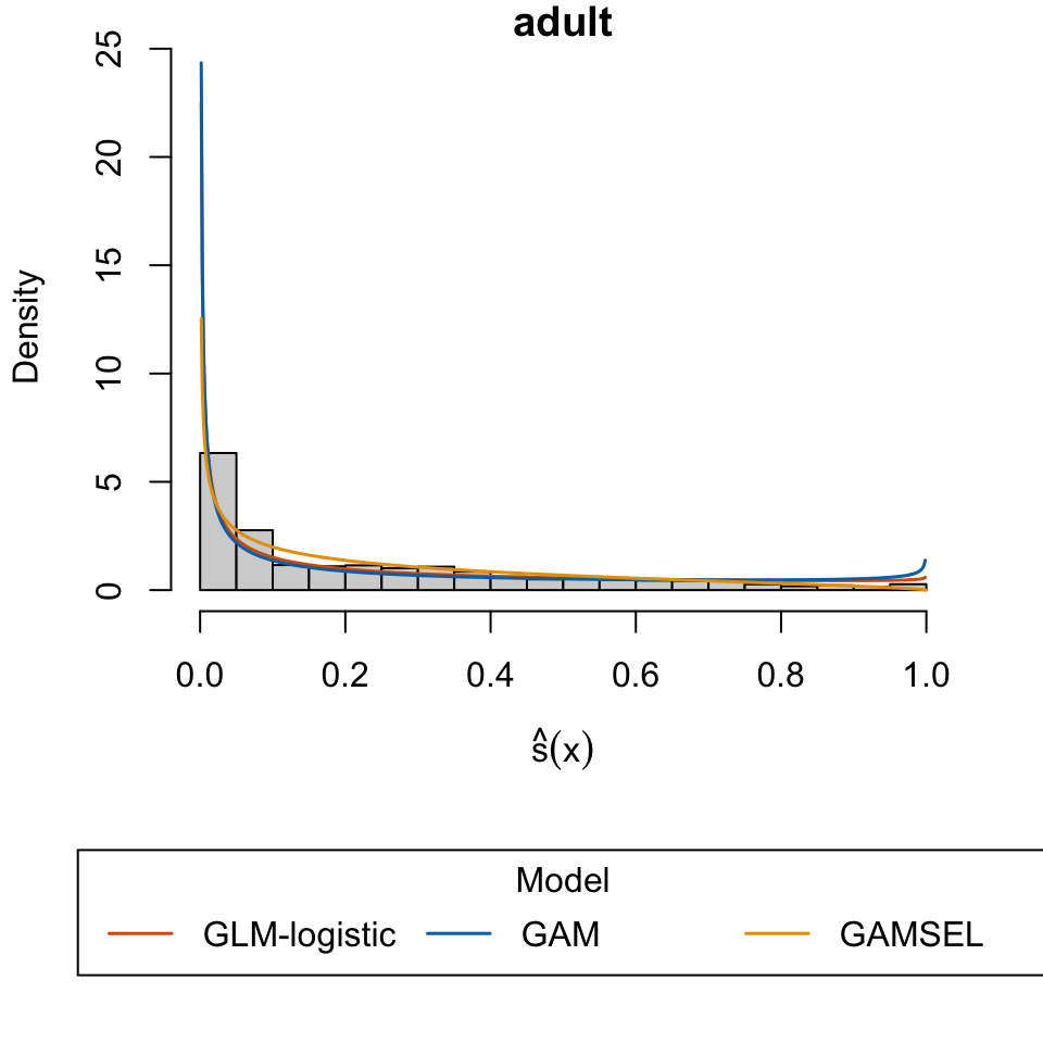
Becker, Barry, and Ronny Kohavi. 1996. “Adult.” UCI Machine Learning Repository.
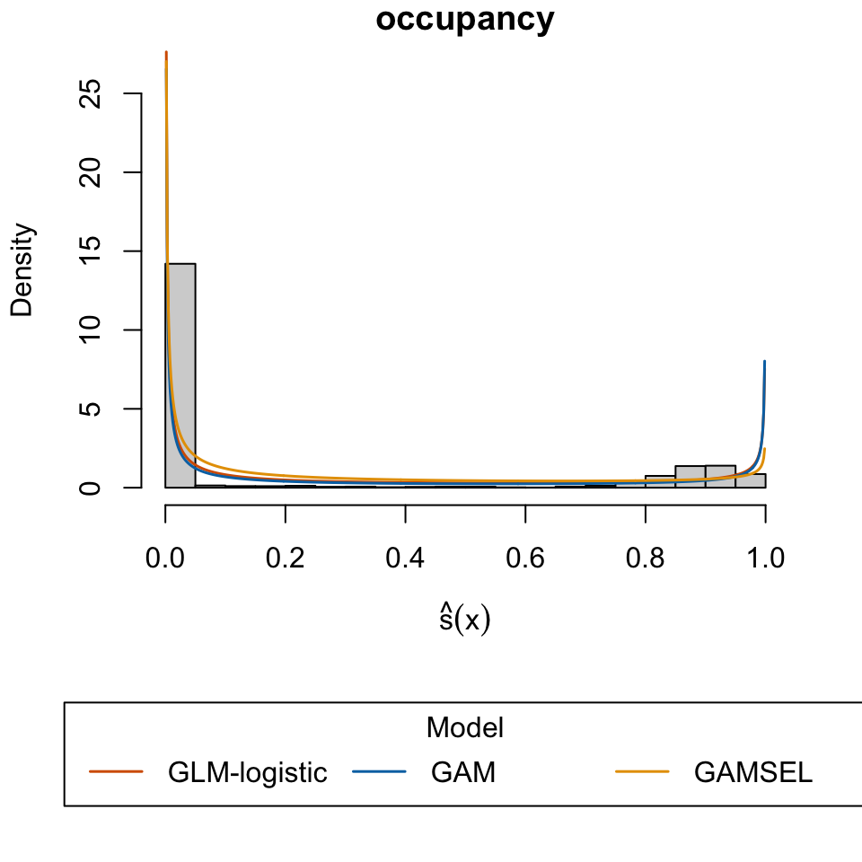
Candanedo, Luis. 2016. “Occupancy Detection .” UCI Machine Learning Repository.
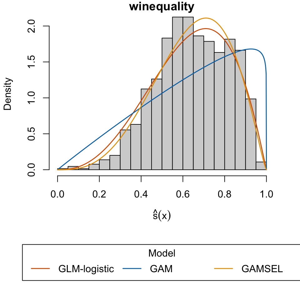
Cortez, Paulo, A. Cerdeira, F. Almeida, T. Matos, and J. Reis. 2009. “Wine Quality.” UCI Machine Learning Repository.
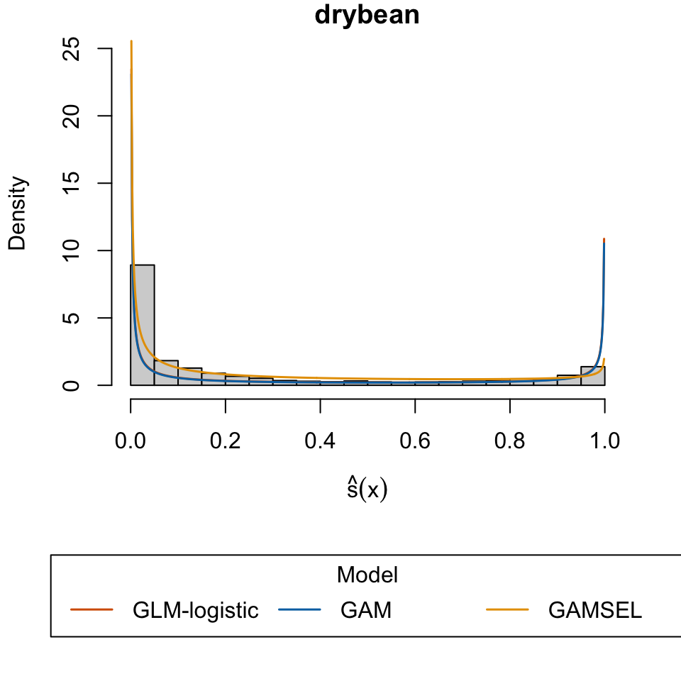
“Dry Bean.” 2020. UCI Machine Learning Repository.
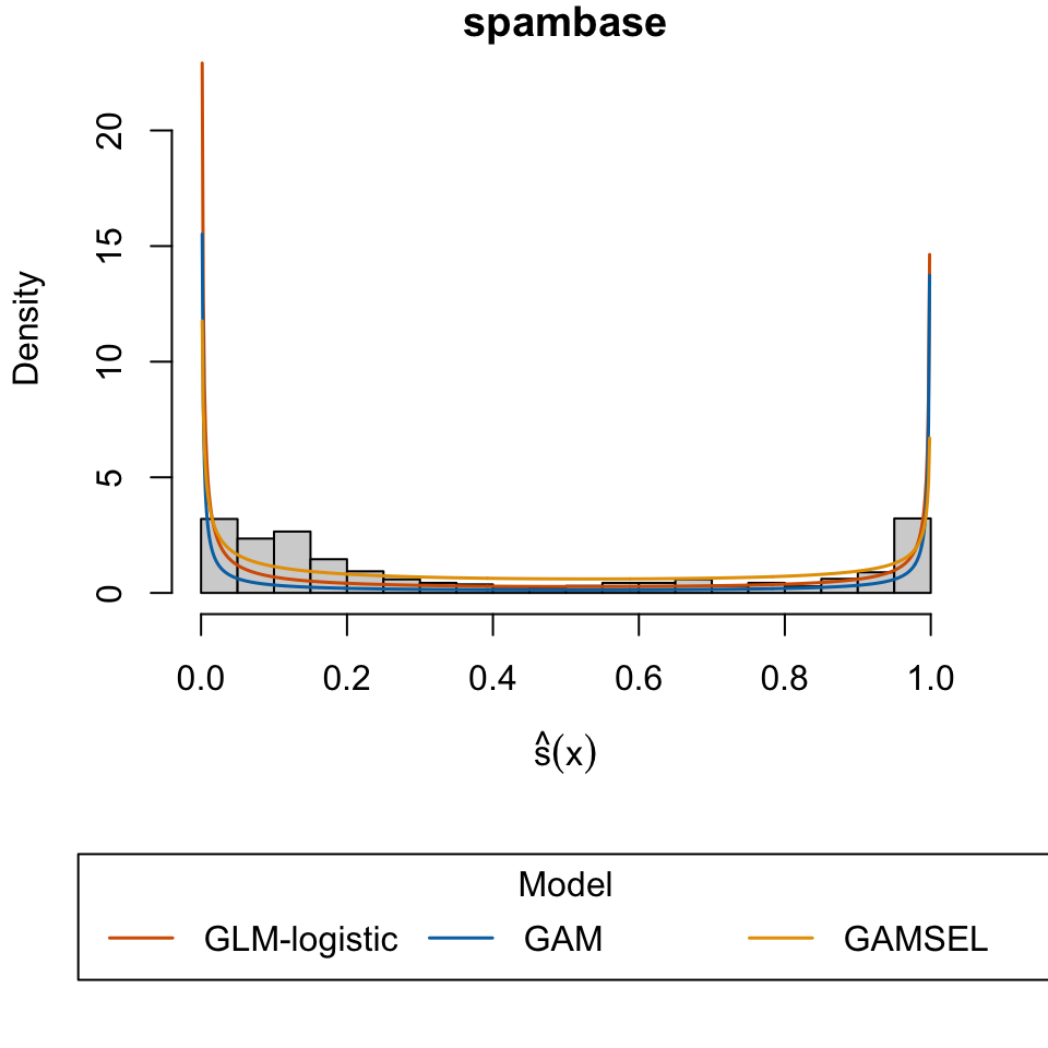
Hopkins, Mark, Erik Reeber, George Forman, and Jaap Suermondt. 1999. “Spambase.” UCI Machine Learning Repository.
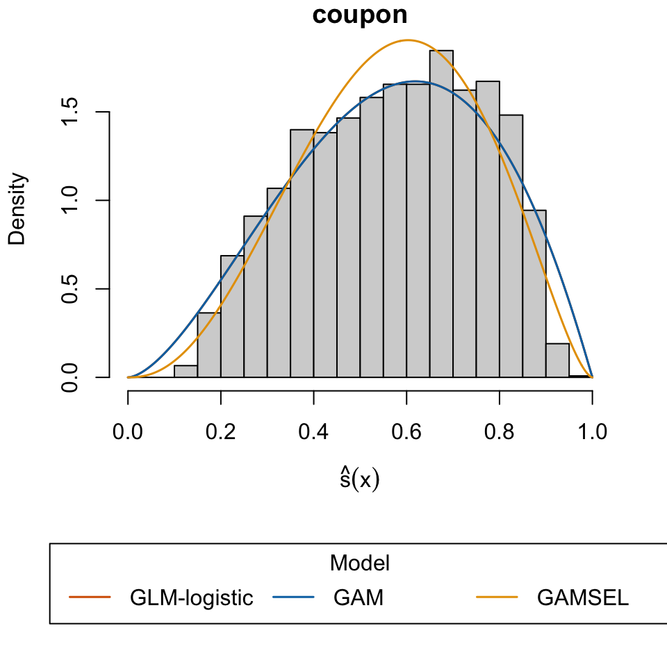
“In-Vehicle Coupon Recommendation.” 2020. UCI Machine Learning Repository.
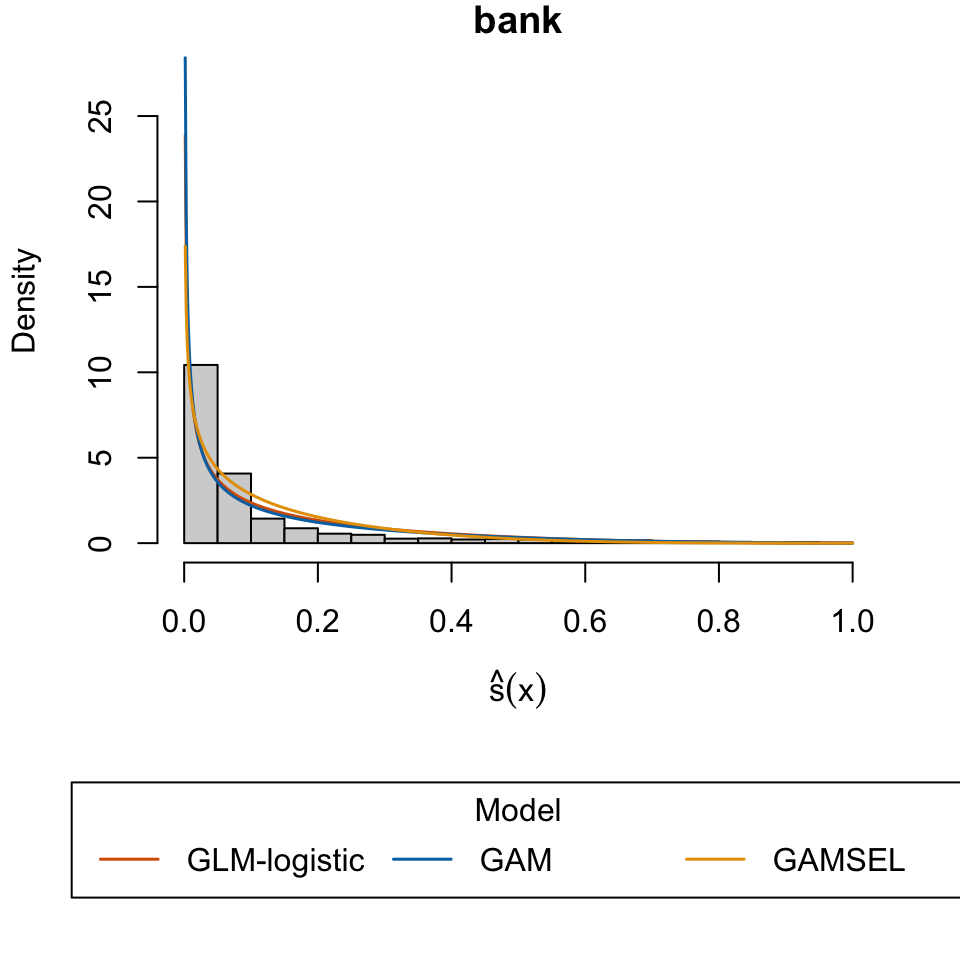
Moro, S., P. Rita, and P. Cortez. 2012. “Bank Marketing.” UCI Machine Learning Repository.
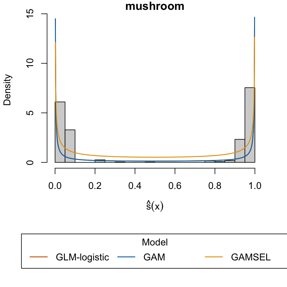
“Mushroom.” 1987. UCI Machine Learning Repository.
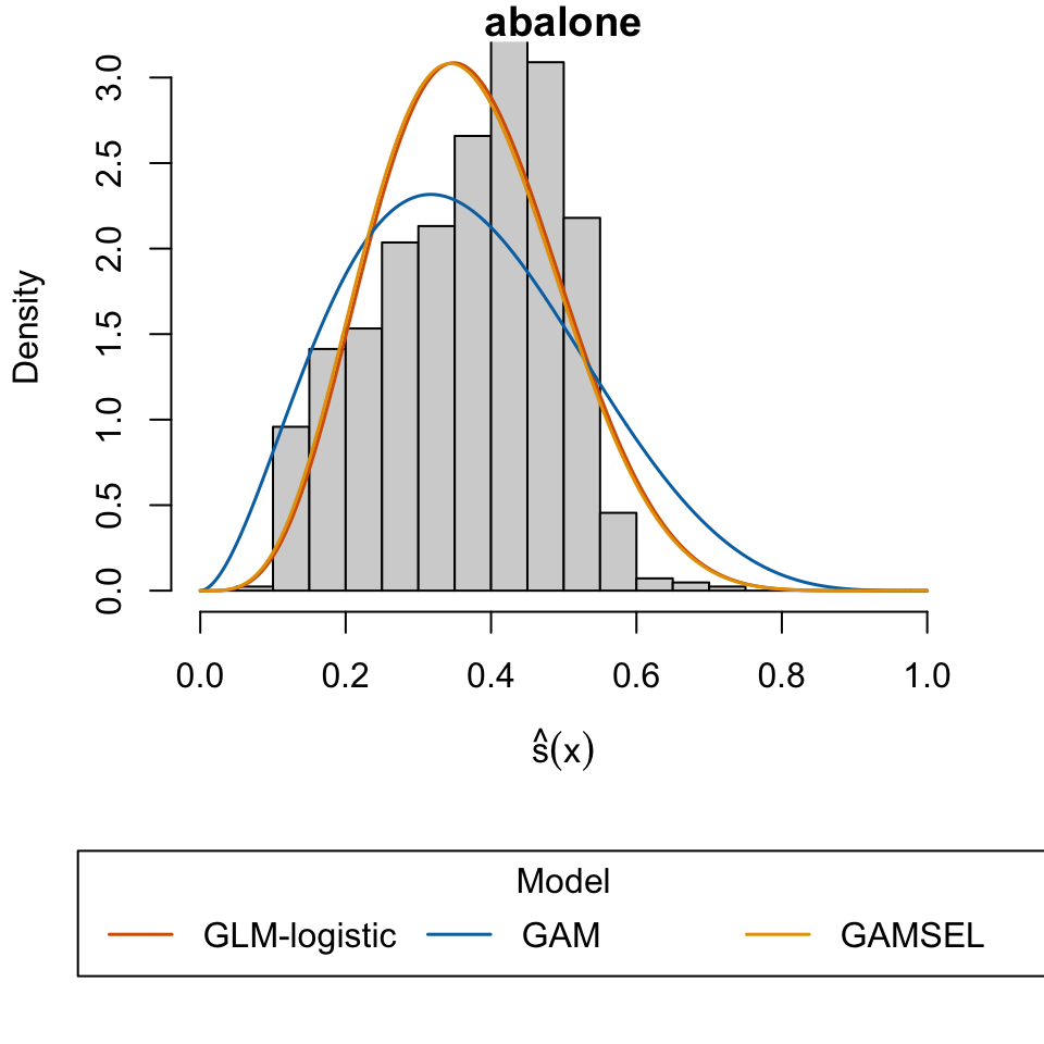
Nash, Warwick, Tracy Sellers, Simon Talbot, Andrew Cawthorn, and Wes Ford. 1995. “Abalone.” UCI Machine Learning Repository.
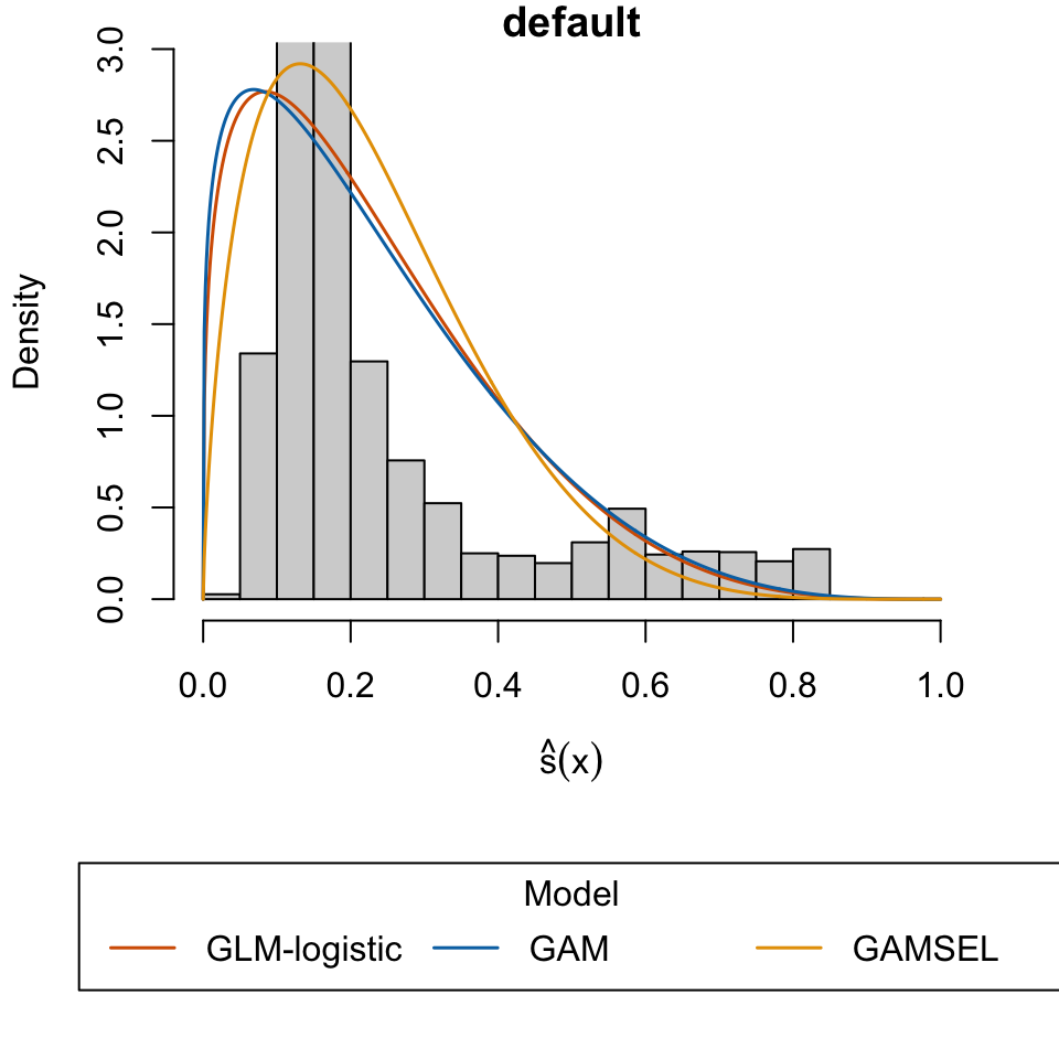
Yeh, I-Cheng. 2016. “Default of Credit Card Clients.” UCI Machine Learning Repository.