16 Results

Note

In this chapter, we display the results from the estimated models from Chapter 15

library(tidyverse)

── Attaching core tidyverse packages ──────────────────────── tidyverse 2.0.0 ──
✔ dplyr     1.1.4     ✔ readr     2.1.5
✔ forcats   1.0.0     ✔ stringr   1.5.1
✔ ggplot2   3.5.1     ✔ tibble    3.2.1
✔ lubridate 1.9.3     ✔ tidyr     1.3.1
✔ purrr     1.0.2     
── Conflicts ────────────────────────────────────────── tidyverse_conflicts() ──
✖ dplyr::filter() masks stats::filter()
✖ dplyr::lag()    masks stats::lag()
ℹ Use the conflicted package (<http://conflicted.r-lib.org/>) to force all conflicts to become errors

library(philentropy)
library(ranger)
library(xgboost)


Attaching package: 'xgboost'

The following object is masked from 'package:dplyr':

    slice

library(pbapply)
library(parallel)

# Colours for train/test
colour_samples <- c(
  "Train" = "#0072B2",
  "Test" = "#D55E00"
)

We define two functions, get_model_interest_rf() and get_model_interest_xgb() to identify, among the estimated models —Random Forest or XGB, respectively— for a given dataset, the hyperparameter set for which a metric is optimal on the test set. The targeted metrics are AUC (performance, to be maximized), ICI (calibration, to be minimized), and the Kullback-Leibler divergence between the estimated scores and the assumed distribution of the underlying probabilities of the binary event. Recall from Chapter 14 that we defined three prior distributions for each dataset, based on parameters of a Beta distribution fitted to scores estimated by GLM, GAM, or GAMSEL models.

Function get_model_interest_rf()

#' From the training results obtained across the grid search of the random
#' forest, extract models of interest (based on scores from test set):
#' max AUC, min ICI, min KL divergence with each of the prior distributions
#'
#' @param resul training results from `simul_xgb_real()`
get_model_interest_rf <- function(resul, tb_metrics, tb_disp_metrics) {

  # Identify best model according to AUC from test set
  ind_max_auc <- tb_metrics |>
    filter(sample == "test") |>
    arrange(desc(AUC)) |>
    pull("ind") |> pluck(1)

  # Identify best model according to Brier score from test set
  ind_min_brier <- tb_metrics |>
    filter(sample == "test") |>
    arrange(brier) |>
    pull("ind") |> pluck(1)
  
  # Identify best model according to ICI from test set
  ind_min_ici <- tb_metrics |>
    filter(sample == "test") |>
    arrange(ici) |>
    pull("ind") |> pluck(1)

  # Identify best model according to KL divergence
  ind_min_kl <- tb_disp_metrics |>
    filter(sample == "test") |>
    group_by(prior) |>
    arrange(KL_20_true_probas) |>
    slice_head(n = 1) |>
    select(model_interest = prior, ind)

  model_of_interest <-
    tibble(model_interest = "max_auc", ind = ind_max_auc) |>
    bind_rows(
      tibble(model_interest = "min_brier", ind = ind_min_brier)
    ) |>
    bind_rows(
      tibble(model_interest = "min_ici", ind = ind_min_ici)
    ) |>
    bind_rows(ind_min_kl)

  model_of_interest |>
    left_join(
      tb_metrics |> select(AUC, brier, ici, sample, ind),
      by = "ind",
      relationship = "many-to-many" # train and test
    ) |>
    left_join(
      tb_disp_metrics |>
        select(
          KL_20_true_probas, inter_quantile_10_90, 
          sample, ind, prior, shape_1, shape_2
        ),
      by = c("ind", "sample", "model_interest" = "prior")
    ) |>
    # Add KL divergence
    left_join(
      tb_disp_metrics |>
        select(
          KL = KL_20_true_probas, quant_ratio = inter_quantile_10_90,
          sample, ind, prior
        ) |>
        pivot_wider(
          names_from = prior,
          values_from = c(KL, quant_ratio)
          # names_glue = "KL_{prior}"
        ),
      by = c("ind", "sample")
    )
}

Function get_model_interest_xgb()

#' From the training results obtained across the grid search of the random
#' forest, extract models of interest (based on scores from test set):
#' max AUC, min ICI, min KL divergence with each of the prior distributions
#'
#' @param resul training results from `simul_xgb_real()`
get_model_interest_xgb <- function(resul, tb_metrics, tb_disp_metrics) {

  # Identify best model according to AUC from test set
  ind_max_auc <- tb_metrics |>
    filter(sample == "validation") |>
    arrange(desc(AUC)) |>
    slice_head(n = 1) |>
    mutate(model_interest = "max_auc") |>
    select(model_interest, ind, nb_iter)

  # Identify best model according to Brier from test set
  ind_min_brier <- tb_metrics |>
    filter(sample == "validation") |>
    arrange(brier) |>
    slice_head(n = 1) |>
    mutate(model_interest = "min_brier") |>
    select(model_interest, ind, nb_iter)
  
  # Identify best model according to ICI from test set
  ind_min_ici <- tb_metrics |>
    filter(sample == "validation") |>
    arrange(ici) |>
    slice_head(n = 1) |>
    mutate(model_interest = "min_ici") |>
    select(model_interest, ind, nb_iter)

  # Identify best model according to KL divergence
  ind_min_kl <- tb_disp_metrics |>
    filter(sample == "validation") |>
    group_by(prior) |>
    arrange(KL_20_true_probas) |>
    slice_head(n = 1) |>
    select(model_interest = prior, ind, nb_iter)

  model_of_interest <-
    ind_max_auc |>
    bind_rows(ind_min_brier) |>
    bind_rows(ind_min_ici) |>
    bind_rows(ind_min_kl)

  model_of_interest |>
    left_join(
      tb_metrics |> select(AUC, brier, ici, sample, ind, nb_iter),
      by = c("ind", "nb_iter"),
      relationship = "many-to-many" # train and test
    ) |>
    left_join(
      tb_disp_metrics |>
        select(
          KL_20_true_probas, inter_quantile_10_90, 
          sample, ind, nb_iter, prior, shape_1, shape_2
        ),
      by = c("ind", "sample", "nb_iter", "model_interest" = "prior")
    ) |>
    # Add KL divergence
    left_join(
      tb_disp_metrics |>
        select(
          KL = KL_20_true_probas, quant_ratio = inter_quantile_10_90, 
          sample, ind, nb_iter, prior
        ) |>
        pivot_wider(
          names_from = prior,
          values_from = c(KL, quant_ratio)
          # names_glue = "KL_{prior}"
        ),
      by = c("ind", "nb_iter", "sample")
    )
}

We also define a third function, get_model_interest_glm() which simply returns the computed metrics for an estimated model.

Function get_model_interest_glm()

#' From the training results obtained for GLM (or GAM, or GAMSEL), extracts
#' AUC, ICI, KL divergence with each of the prior distributions
#'
#' @param resul training results from `simul_xgb_real()`
get_model_interest_glm <- function(resul) {
  resul$tb_metrics |> 
    mutate(model_interest = "none") |> 
    left_join(
      resul$tb_disp_metrics |> 
        select(
          KL = KL_20_true_probas, quant_ratio = inter_quantile_10_90, 
          sample, prior
        ),
      by = "sample"
    ) |> 
    pivot_wider(
      names_from = "prior", 
      values_from = c(KL, quant_ratio)
      # names_glue = "KL_{prior}"
    )
}

We define a wrapper function, get_model_interest(), which calls either get_model_interest_rf(), get_model_interest_xgb(), or get_model_interest_glm() based on whether it receives a list of estimated forests or a list of estimated XGB models.

Function get_model_interest()

#' From the training results obtained across the grid search, extract
#' models of interest (based on scores from test set): max AUC, min ICI,
#' min KL divergence with each of the prior distributions
#'
#' @param resul training results from `simul_xgb_real()`
get_model_interest <- function(resul, 
                               model_type = c("rf", "xgb", "glm", "gam", "gamsel")) {
  tb_metrics <- map(resul$res, "tb_metrics") |> list_rbind()
  tb_disp_metrics <- map(resul$res, "tb_disp_metrics") |> list_rbind()
  if (model_type == "rf") {
    res <- get_model_interest_rf(resul, tb_metrics, tb_disp_metrics)
  } else if (model_type == "xgb") {
    res <- get_model_interest_xgb(resul, tb_metrics, tb_disp_metrics)
  } else {
    res <- get_model_interest_glm(resul)
  }
  res |> mutate(model_type = !!model_type)
}

We define a function, get_row_table(), which retrieves the computed metrics (AUC, ICI, and KL divergence) for the models of interest for a specific dataset:

the model achieving the maximum AUC (AUC*)
the model achieving the minimum ICI (ICI*)
the model minimizing the KL divergence between the scores and the Beta distribution, where parameters are estimated using scores from a GLM model (\(\text{KL}^{GLM}\))
the model minimizing the KL divergence between the scores and the Beta distribution, where parameters are estimated using scores from a GAM model (\(\text{KL}^{GAM}\))
the model minimizing the KL divergence between the scores and the Beta distribution, where parameters are estimated using scores from a GAMSEL model (\(\text{KL}^{GAMSEL}\))”

For the models represented by \(\text{KL}^{GLM}\), \(\text{KL}^{GAM}\), and \(\text{KL}^{GAMSEL}\), we also compute the changes in AUC (\(\Delta AUC\)), Brier (\(\Delta Brier\)), ICI (\(\Delta ICI\)), and KL divergence (\(\Delta KL\)) relative to the metrics obtained from the model where the AUC is maximized.

Function get_row_table()

#' @param model_interest computed metrics for the model of interest
#' @param name name of the dataset
get_row_table <- function(model_interest, name) {
  model_interest |>
    filter(sample == "test") |>
    select(
      model_type, model_interest, AUC, brier, ici, 
      quant_ratio_glm, quant_ratio_gam, quant_ratio_gamsel,
      KL = KL_20_true_probas, 
      KL_glm, KL_gam, KL_gamsel
    ) |>
    mutate(dataset = !!name) |>
    pivot_wider(
      names_from = "model_interest",
      values_from = c(
        "AUC", "brier", "ici", "KL", 
        "quant_ratio_glm", "quant_ratio_gam", "quant_ratio_gamsel",
        "KL_glm", "KL_gam", "KL_gamsel"
      )
    ) |>
    mutate(
      # variation in AUC
      diff_auc_glm = AUC_glm - AUC_max_auc,
      diff_auc_gam = AUC_gam - AUC_max_auc,
      diff_auc_gamsel = AUC_gamsel - AUC_max_auc,
      # variation in Brier score
      diff_brier_glm = brier_glm - brier_max_auc,
      diff_brier_gam = brier_gam - brier_max_auc,
      diff_brier_gamsel = brier_gamsel - brier_max_auc,
      # variation in ICI
      diff_ici_glm = ici_glm - ici_max_auc,
      diff_ici_gam = ici_gam - ici_max_auc,
      diff_ici_gamsel = ici_gamsel - ici_max_auc,
      # variation in KL divergence
      diff_kl_glm = KL_glm_glm - KL_glm_max_auc,
      diff_kl_gam = KL_gam_gam - KL_gam_max_auc,
      diff_kl_gamsel = KL_gamsel_gamsel - KL_gamsel_max_auc
    )
}

For the GLM, GAM, and GAMSEL models, we only report the metrics calculated for each model.

Function get_row_table_glm()

get_row_table_glm <- function(model_glms, name) {
  model_glms |>
    filter(sample == "test") |>
    select(
      model_type, model_interest, AUC, brier, ici,
      quant_ratio_glm, quant_ratio_gam, quant_ratio_gamsel,
      KL_glm, KL_gam, KL_gamsel
    ) |>
    mutate(
      dataset = !!name,
      tmp = model_type
    ) |>
    rename(
      KL_glm_glm = KL_glm,
      KL_gam_gam = KL_gam,
      KL_gamsel_gamsel = KL_gamsel,
      quant_ratio_glm_glm = quant_ratio_glm,
      quant_ratio_gam_gam = quant_ratio_gam,
      quant_ratio_gamsel_gamsel = quant_ratio_gamsel
    ) |> 
    mutate(
      AUC_glm = AUC,
      AUC_gam = AUC,
      AUC_gamsel = AUC,
      brier_glm = brier,
      brier_gam = brier,
      brier_gamsel = brier,
      ici_glm = ici,
      ici_gam = ici,
      ici_gamsel = ici
    ) |> 
    select(-AUC, -brier, -ici)
}

16.1 Estimated Metrics

We loop over the results obtained from Chapter 15 to extract the metrics.

datasets <- tribble(
  ~name, ~target_name,
  "abalone", "Sex",
  "adult", "high_income",
  "bank", "y",
  "default", "default",
  "drybean", "is_dermason",
  "coupon", "y",
  "mushroom", "edible",
  "occupancy", "Occupancy",
  "winequality", "high_quality",
  "spambase", "is_spam"
)
result_table <- vector(mode = "list", length = nrow(datasets))
priors <- vector(mode = "list", length = nrow(datasets))
names(priors) <- datasets$name
scores_hist <- list()
for (i_model in 1:nrow(datasets)) {
  name <- datasets$name[i_model]
  # Load priors
  load(str_c("output/real-data/priors_", name, ".rda"))
  priors[[i_model]] <- get(str_c("priors_", name))
  # Load results
  load(str_c("output/real-data/rf_resul_", name, ".rda"))
  load(str_c("output/real-data/xgb_resul_", name, ".rda"))
  model_interest <-
    get_model_interest(resul = rf_resul, model_type = "rf") |>
    bind_rows(get_model_interest(resul = xgb_resul, model_type = "xgb"))
  result_table_ml <- get_row_table(model_interest = model_interest, name = name)
  
  load(str_c("output/real-data/glm_resul_", name, ".rda"))
  load(str_c("output/real-data/gam_resul_", name, ".rda"))
  load(str_c("output/real-data/gamsel_resul_", name, ".rda"))
  model_glms <- get_model_interest(resul = glm_resul, model_type = "glm") |> 
    bind_rows(get_model_interest(resul = gam_resul, model_type = "gam")) |> 
    bind_rows(get_model_interest(resul = gamsel_resul, model_type = "gamsel"))
  result_table_gl <- get_row_table_glm(model_glms = model_glms, name = name)
  
  result_table[[i_model]] <- result_table_ml |> bind_rows(result_table_gl)

  tb_ind_model_interest <- 
    model_interest |> filter(sample == "test") |> 
    select(model_interest, model_type, ind)
  
  # Extract histograms for model of interest
  scores_hist_current <- list()
  for (model in c("rf", "xgb")) {
    scores_hist_current_model <- 
      tb_ind_model_interest |> 
      filter(model_type == model) |> 
      pull("ind") |> 
      map(~rf_resul$res[[.x]]$scores_hist)
    for (j in 1:length(scores_hist_current_model)) {
      scores_hist_current_model[[j]]$model_interest <- 
        tb_ind_model_interest |> 
        filter(model_type == !!model) |> 
        pull(model_interest) |> pluck(j)
      scores_hist_current_model[[j]]$model_type <- model
      scores_hist_current_model[[j]]$name <- name
    }
    scores_hist_current <- c(scores_hist_current, scores_hist_current_model)
  }
  scores_hist <- c(scores_hist, scores_hist_current)
}

Codes to create result tables

red_colours <- c(
  "#FFD6D6", "#FFCCCC", "#FFC2C2", "#FFB8B8", "#FFADAD", 
  "#FFA3A3", "#FF9999", "#FF8F8F", "#FF8585", "#FF7A7A"
)
red_colours_txt <- c(
  "#333333", "#333333", "#2B2B2B", "#2B2B2B", "#232323", 
  "#1F1F1F", "#1A1A1A", "#141414", "#101010", "#0A0A0A"
)
green_colours <- c(
  "#E9F6E9", "#D4F2D4", "#BFEFBF", "#AADCA9", "#96C996",
  "#81B781", "#6CA56C", "#578252", "#426F42", "#2F5D2F"
)
green_colours_txt <- c(
  "#1A1A1A", "#1A1A1A", "#1A1A1A", "#1A1A1A", "#1A1A1A",
  "#E6E6E6", "#E6E6E6", "#E6E6E6", "#E6E6E6", "#E6E6E6"
)

accuracy_digits <- 0.01

get_range_for_colours <- function(variable_name, table_kb) {
  value <- table_kb |> 
    # filter(value_type == "mean") |> 
    pull(!!variable_name) |> 
    range(na.rm = TRUE) |> abs() |> max()
  value * c(-1, 1)
}

get_colour <- function(variable, value_type, min_or_max, colour_type, table_kb) {
  variable_string <- deparse(substitute(variable))
  if (colour_type == "bg") {
    # background colour
    if (min_or_max == "min") {
      colours <- rev(c(rev(red_colours), green_colours))
    } else {
      colours <- c(rev(red_colours), rev(green_colours))
    }
  } else {
    # text colour
    if (min_or_max == "min") {
      colours <- rev(c(rev(red_colours_txt), green_colours_txt))
    } else {
      colours <- c(rev(red_colours_txt), rev(green_colours_txt))
    }
  }
  kableExtra::spec_color(
    variable,
    palette = colours,
    scale_from = get_range_for_colours(variable_string, table_kb = table_kb),
    na_color = "white"
  )
}

print_table <- function(format, 
                        table_kb, 
                        prior_model = c("glm", "gam", "gamsel")) {
  tb_with_colours <- table_kb |> 
    rowwise() |> 
    mutate(
      # When min KL
      ## Delta AUC
      diff_auc_bgcol = get_colour(
        !!sym(str_c("diff_auc_", prior_model)), value_type, "max", "bg", table_kb
      ),
      diff_auc_txtcol = get_colour(
        !!sym(str_c("diff_auc_", prior_model)), value_type, "max", "txt", table_kb
      ),
      ## Delta Brier
      diff_brier_bgcol = get_colour(
        !!sym(str_c("diff_brier_", prior_model)), value_type, "min", "bg", table_kb
      ),
      diff_brier_txtcol = get_colour(
        !!sym(str_c("diff_brier_", prior_model)), value_type, "min", "txt", table_kb
      ),
      ## Delta ICI
      diff_ici_bgcol = get_colour(
        !!sym(str_c("diff_ici_", prior_model)), value_type, "min", "bg", table_kb
      ),
      diff_ici_txtcol = get_colour(
        !!sym(str_c("diff_ici_", prior_model)), value_type, "min", "txt", table_kb
      ),
      ## Delta KL
      diff_kl_bgcol = get_colour(
        !!sym(str_c("diff_kl_", prior_model)), value_type, "min", "bg", table_kb
      ),
      diff_kl_txtcol = get_colour(
        !!sym(str_c("diff_kl_", prior_model)), value_type, "min", "txt", table_kb
      ),
    )
  
  table_kb |> 
     mutate(
      across(
        where(is.numeric), 
        ~scales::number(.x, accuracy = accuracy_digits)
      )
    ) |> 
    knitr::kable(
      col.names = c(
        "Dataset", "Model",
        "AUC", "brier", "ICI", "KL", "Quant. Ratio", # model with max AUC
        "AUC", "brier", "ICI", "KL", "Quant. Ratio", # model with min Brier
        "AUC", "brier", "ICI", "KL", "Quant. Ratio", # model with min ICI
        "AUC", "brier", "ICI", "KL", "Quant. Ratio", "ΔAUC", "ΔBrier", "ΔICI", "ΔKL"
      ),
      escape = FALSE, booktabs = T, digits = 3, format = format) |>
    ## Delta AUC
    kableExtra::column_spec(
      which(colnames(table_kb) == str_c("diff_auc_", prior_model)),
      background = tb_with_colours$diff_auc_bgcol,
      color = tb_with_colours$diff_auc_txtcol
    ) |>
    ## Delta Brier
    kableExtra::column_spec(
      which(colnames(table_kb) == str_c("diff_brier_", prior_model)),
      background = tb_with_colours$diff_brier_bgcol,
      color = tb_with_colours$diff_brier_txtcol
    ) |>
    ## Delta ICI
    kableExtra::column_spec(
      which(colnames(table_kb) == str_c("diff_ici_", prior_model)),
      background = tb_with_colours$diff_ici_bgcol,
      color = tb_with_colours$diff_ici_txtcol
    ) |>
    ## Delta KL
    kableExtra::column_spec(
      which(colnames(table_kb) == str_c("diff_kl_", prior_model)),
      background = tb_with_colours$diff_kl_bgcol,
      color = tb_with_colours$diff_kl_txtcol
    ) |>
    kableExtra::collapse_rows(columns = 1:2, valign = "top") |>
    kableExtra::add_header_above(
      c(" " = 2,
        "AUC*" = 5,
        "Brier*" = 5,
        "ICI*" = 5,
        "KL*" = 9
      )
    )
}

opts <- options(knitr.kable.NA = "")

The estimated metrics for the GLM, GAM, and GAMSEL:

Codes to create the table

tbl_kb <- result_table |>
  list_rbind() |>
  filter(model_type %in% c("glm", "gam", "gamsel")) |> 
  select(
    dataset, model_type,
    AUC_glm, brier_glm, ici_glm,
    quant_ratio_glm_glm, quant_ratio_gam_gam, quant_ratio_gamsel_gamsel,
    KL_glm_glm, KL_gam_gam, KL_gamsel_gamsel
  ) |>
  mutate(
    model_type = factor(
      model_type, 
      levels = c("glm", "gam", "gamsel"), 
      labels = c("GLM", "GAM", "GAMSEL")
    )
  ) |> 
  mutate(
    across(
      where(is.numeric), 
      ~scales::number(.x, accuracy = accuracy_digits)
    )
  )

cbind(
  tbl_kb |> filter(dataset %in% datasets$name[1:5]),
  tbl_kb |> filter(dataset %in% datasets$name[6:10])
) |> 
  knitr::kable(
    col.names = c(
      rep(c("Dataset","Model",
      "AUC", "brier", "ICI",
      "QR-GLM", "QR-GAM", "QR-GAMSEL",
      "KL-GLM", "KL-GAM", "KL-GAMSEL"
      ), 2)
    ),
    escape = FALSE, booktabs = T, digits = 3, format = "markdown") |>
  kableExtra::collapse_rows(columns = c(1, 12), valign = "top")

Dataset	Model	AUC	brier	ICI	QR-GLM	QR-GAM	QR-GAMSEL	KL-GLM	KL-GAM	KL-GAMSEL	Dataset	Model	AUC	brier	ICI	QR-GLM	QR-GAM	QR-GAMSEL	KL-GLM	KL-GAM	KL-GAMSEL
abalone	GLM	0.70	0.20	0.06	1.06	0.81	1.06	0.05	0.11	0.05	coupon	GLM	0.75	0.20	0.01	1.05	1.05	1.17	0.02	0.02	0.06
	GAM	0.71	0.20	0.02	1.27	0.96	1.26	0.32	0.13	0.30		GAM	0.75	0.20	0.01	1.05	1.05	1.17	0.02	0.02	0.06
	GAMSEL	0.71	0.20	0.04	1.09	0.83	1.09	0.11	0.17	0.10		GAMSEL	0.75	0.20	0.02	0.94	0.94	1.05	0.05	0.05	0.03
adult	GLM	0.90	0.10	0.00	0.92	0.86	1.13	0.02	0.02	0.16	mushroom	GLM	1.00	0.00	0.00	1.00	1.00	1.02	0.29	0.29	1.40
	GAM	0.91	0.10	0.01	0.96	0.90	1.18	0.05	0.03	0.23		GAM	1.00	0.00	0.00	1.00	1.00	1.02	0.29	0.29	1.40
	GAMSEL	0.90	0.11	0.03	0.81	0.76	1.00	0.06	0.10	0.05		GAMSEL	1.00	0.01	0.04	0.94	0.94	0.96	0.61	0.61	0.90
bank	GLM	0.91	0.07	0.03	0.83	0.84	1.00	0.20	0.15	0.32	occupancy	GLM	1.00	0.01	0.01	1.02	1.01	1.13	0.46	0.35	0.85
	GAM	0.92	0.07	0.02	0.92	0.93	1.10	0.20	0.14	0.34		GAM	1.00	0.01	0.01	1.02	1.02	1.14	0.50	0.38	0.92
	GAMSEL	0.91	0.07	0.03	0.78	0.79	0.94	0.13	0.10	0.20		GAMSEL	0.99	0.02	0.04	0.93	0.93	1.04	0.41	0.34	0.63
default	GLM	0.77	0.14	0.02	1.09	1.06	1.23	0.45	0.45	0.49	winequality	GLM	0.74	0.20	0.04	0.97	0.75	1.03	0.06	0.22	0.06
	GAM	0.78	0.13	0.01	1.13	1.10	1.27	0.29	0.28	0.35		GAM	0.79	0.18	0.04	1.22	0.95	1.30	0.14	0.02	0.21
	GAMSEL	0.76	0.14	0.03	0.94	0.92	1.07	0.73	0.75	0.70		GAMSEL	0.75	0.20	0.04	0.92	0.72	0.99	0.04	0.24	0.03
drybean	GLM	0.99	0.03	0.01	1.00	1.00	1.16	0.06	0.05	0.57	spambase	GLM	0.97	0.06	0.02	1.00	1.00	1.05	0.02	0.15	0.37
	GAM	0.99	0.03	0.01	1.00	1.00	1.17	0.08	0.07	0.64		GAM	0.91	0.08	0.07	1.00	1.00	1.05	0.67	0.29	1.69
	GAMSEL	0.99	0.04	0.06	0.91	0.91	1.06	0.19	0.21	0.06		GAMSEL	0.96	0.07	0.06	0.96	0.96	1.01	0.44	0.98	0.18

Codes to create the table

result_table_glm <- 
  result_table |>
  list_rbind() |>
  filter(model_type %in% c("rf", "xgb")) |> 
  select(
    dataset, model_type,
    # model with max AUC
    AUC_max_auc, brier_max_auc, ici_max_auc, KL_glm_max_auc, quant_ratio_glm_max_auc,
    # model with min Brier
    AUC_min_brier, brier_min_brier, ici_min_brier, KL_glm_min_brier, quant_ratio_glm_min_brier,
    # model with min ICI
    AUC_min_ici, brier_min_ici, ici_min_ici, KL_glm_min_ici, quant_ratio_glm_min_ici,
    # model with min KL distance with prior from GLM
    AUC_glm, brier_glm, ici_glm, KL_glm_glm, quant_ratio_glm_glm,
    diff_auc_glm, diff_brier_glm, diff_ici_glm, diff_kl_glm 
  ) |>
  mutate(
    model_type = factor(
      model_type, 
      levels = c("rf", "xgb", "glm", "gam", "gamsel"), 
      labels = c("RF", "XGB", "GLM", "GAM", "GAMSEL")
    )
  )

print_table(
  format = "markdown", table_kb = result_table_glm, prior_model = "glm"
)

Table 16.1: Comparison of metrics for models chosen based on AUC, on AIC, or on KL divergence with a prior on the distribution of the probabilities estimated with a GLM.

		AUC*					Brier*					ICI*					KL*
Dataset	Model	AUC	brier	ICI	KL	Quant. Ratio	AUC	brier	ICI	KL	Quant. Ratio	AUC	brier	ICI	KL	Quant. Ratio	AUC	brier	ICI	KL	Quant. Ratio	ΔAUC	ΔBrier	ΔICI	ΔKL
abalone	RF	0.71	0.20	0.03	0.34	1.21	0.71	0.20	0.03	0.34	1.24	0.51	0.23	0.02	2.73	0.00	0.71	0.20	0.03	0.33	1.28	0.00	0.00	0.00	-0.01
abalone	XGB	0.69	0.20	0.03	0.42	1.45	0.69	0.20	0.04	0.56	1.06	0.70	0.20	0.04	0.80	1.03	0.69	0.21	0.05	0.24	1.23	0.00	0.00	0.02	-0.18
adult	RF	0.92	0.10	0.03	0.03	0.88	0.92	0.10	0.03	0.02	0.89	0.51	0.18	0.00	4.46	0.00	0.92	0.10	0.03	0.02	0.89	0.00	0.00	0.00	-0.01
adult	XGB	0.93	0.09	0.01	0.09	1.00	0.93	0.09	0.01	0.09	1.00	0.93	0.09	0.01	0.09	0.97	0.91	0.10	0.02	0.04	0.90	-0.01	0.01	0.01	-0.05
bank	RF	0.94	0.06	0.02	0.19	1.08	0.94	0.06	0.02	0.21	1.10	0.94	0.06	0.02	0.21	1.12	0.92	0.07	0.04	0.07	0.82	-0.02	0.01	0.02	-0.12
bank	XGB	0.93	0.06	0.02	0.36	1.17	0.93	0.06	0.02	0.28	1.12	0.93	0.06	0.02	0.34	1.15	0.91	0.07	0.03	0.07	0.93	-0.02	0.00	0.01	-0.29
default	RF	0.78	0.13	0.02	0.20	1.10	0.78	0.13	0.01	0.18	1.12	0.78	0.13	0.01	0.16	1.15	0.77	0.14	0.02	0.13	1.17	-0.02	0.00	0.00	-0.07
default	XGB	0.78	0.13	0.01	0.23	1.17	0.78	0.13	0.01	0.29	1.15	0.78	0.13	0.01	0.22	1.19	0.77	0.13	0.01	0.19	1.17	-0.01	0.00	0.00	-0.04
drybean	RF	0.99	0.03	0.01	0.06	1.00	0.99	0.03	0.01	0.07	1.00	0.99	0.03	0.01	0.06	1.00	0.99	0.03	0.02	0.02	0.98	0.00	0.00	0.01	-0.04
drybean	XGB	0.99	0.03	0.01	0.08	1.00	0.99	0.03	0.01	0.09	1.00	0.99	0.03	0.01	0.09	1.00	0.99	0.03	0.04	0.07	0.92	0.00	0.00	0.03	-0.02
coupon	RF	0.83	0.17	0.07	0.04	0.98	0.83	0.17	0.07	0.04	0.98	0.51	0.24	0.00	3.60	0.00	0.83	0.17	0.07	0.04	0.98	0.00	0.00	0.00	0.00
coupon	XGB	0.84	0.17	0.10	2.27	1.74	0.84	0.16	0.03	0.81	1.53	0.83	0.16	0.02	0.37	1.39	0.78	0.19	0.03	0.04	1.03	-0.06	0.02	-0.07	-2.23
mushroom	RF	1.00	0.01	0.05	0.23	0.96	1.00	0.00	0.01	0.22	1.00	1.00	0.00	0.01	0.22	1.00	1.00	0.01	0.04	0.11	0.99	0.00	0.00	-0.02	-0.12
mushroom	XGB	1.00	0.00	0.00	0.28	1.00	1.00	0.00	0.00	0.29	1.00	1.00	0.00	0.00	0.28	1.00	1.00	0.01	0.04	0.13	0.97	0.00	0.01	0.03	-0.15
occupancy	RF	1.00	0.01	0.00	0.56	1.04	1.00	0.01	0.00	0.57	1.04	1.00	0.01	0.00	0.57	1.04	1.00	0.01	0.04	0.31	0.97	0.00	0.01	0.03	-0.25
occupancy	XGB	1.00	0.01	0.01	0.60	1.04	1.00	0.01	0.01	0.66	1.04	1.00	0.01	0.00	0.54	1.03	1.00	0.01	0.04	0.47	0.95	0.00	0.00	0.04	-0.13
winequality	RF	0.89	0.14	0.07	0.32	1.42	0.89	0.13	0.03	0.69	1.58	0.51	0.24	0.03	3.43	0.00	0.84	0.17	0.08	0.05	1.07	-0.05	0.03	0.01	-0.27
winequality	XGB	0.87	0.15	0.12	4.06	1.97	0.86	0.14	0.04	1.63	1.75	0.83	0.17	0.03	0.35	1.39	0.80	0.18	0.04	0.11	1.12	-0.07	0.03	-0.08	-3.96
spambase	RF	0.99	0.05	0.06	0.21	0.96	0.99	0.04	0.04	0.10	0.98	0.51	0.24	0.01	6.08	0.00	0.99	0.04	0.04	0.10	0.98	0.00	0.00	-0.02	-0.11
spambase	XGB	0.98	0.04	0.01	0.23	1.00	0.99	0.04	0.01	0.17	1.00	0.99	0.04	0.01	0.17	1.00	0.98	0.04	0.01	0.10	0.99	0.00	0.01	0.00	-0.13

Codes to create the table

result_table_gam <- 
  result_table |>
  list_rbind() |>
  filter(model_type %in% c("rf", "xgb")) |> 
  select(
    dataset, model_type,
    # model with max AUC
    AUC_max_auc, brier_max_auc, ici_max_auc, KL_gam_max_auc, quant_ratio_gam_max_auc,
    # model with min Brier
    AUC_min_brier, brier_min_brier, ici_min_brier, quant_ratio_gam_min_brier, KL_gam_min_brier,
    # model with min ICI
    AUC_min_ici, brier_min_ici, ici_min_ici, KL_gam_min_ici, quant_ratio_gam_min_ici,
    # model with min KL distance with prior from GAM
    AUC_gam, brier_gam, ici_gam, KL_gam_gam, quant_ratio_gam_gam,
    diff_auc_gam, diff_brier_gam, diff_ici_gam, diff_kl_gam 
  ) |>
  mutate(
    model_type = factor(
      model_type, 
      levels = c("rf", "xgb", "glm", "gam", "gamsel"), 
      labels = c("RF", "XGB", "GLM", "GAM", "GAMSEL")
    )
  )


print_table(
  format = "markdown", table_kb = result_table_gam, prior_model = "gam"
)

Table 16.2: Comparison of metrics for models chosen based on AUC, on AIC, or on KL divergence with a prior on the distribution of the probabilities estimated with a GAM.

		AUC*					Brier*					ICI*					KL*
Dataset	Model	AUC	brier	ICI	KL	Quant. Ratio	AUC	brier	ICI	KL	Quant. Ratio	AUC	brier	ICI	KL	Quant. Ratio	AUC	brier	ICI	KL	Quant. Ratio	ΔAUC	ΔBrier	ΔICI	ΔKL
abalone	RF	0.71	0.20	0.03	0.24	0.92	0.71	0.20	0.03	0.94	0.21	0.51	0.23	0.02	3.18	0.00	0.70	0.20	0.04	0.13	1.07	-0.01	0.00	0.01	-0.11
abalone	XGB	0.69	0.20	0.03	0.12	1.11	0.69	0.20	0.04	0.80	0.58	0.70	0.20	0.04	0.92	0.78	0.69	0.21	0.04	0.14	1.26	0.00	0.00	0.01	0.02
adult	RF	0.92	0.10	0.03	0.06	0.83	0.92	0.10	0.03	0.83	0.04	0.51	0.18	0.00	4.63	0.00	0.92	0.10	0.03	0.04	0.83	0.00	0.00	0.00	-0.01
adult	XGB	0.93	0.09	0.01	0.06	0.93	0.93	0.09	0.01	0.93	0.06	0.93	0.09	0.01	0.06	0.91	0.92	0.09	0.01	0.05	0.88	-0.01	0.00	0.01	-0.02
bank	RF	0.94	0.06	0.02	0.14	1.09	0.94	0.06	0.02	1.11	0.15	0.94	0.06	0.02	0.15	1.13	0.92	0.07	0.04	0.05	0.87	-0.01	0.01	0.02	-0.08
bank	XGB	0.93	0.06	0.02	0.28	1.18	0.93	0.06	0.02	1.13	0.21	0.93	0.06	0.02	0.26	1.16	0.91	0.07	0.03	0.05	0.96	-0.02	0.00	0.01	-0.23
default	RF	0.78	0.13	0.02	0.20	1.07	0.78	0.13	0.01	1.09	0.17	0.78	0.13	0.01	0.15	1.12	0.77	0.14	0.02	0.12	1.14	-0.02	0.00	0.00	-0.08
default	XGB	0.78	0.13	0.01	0.22	1.14	0.78	0.13	0.01	1.12	0.29	0.78	0.13	0.01	0.20	1.16	0.77	0.13	0.01	0.17	1.14	-0.01	0.00	0.00	-0.05
drybean	RF	0.99	0.03	0.01	0.05	1.00	0.99	0.03	0.01	1.00	0.06	0.99	0.03	0.01	0.05	1.00	0.99	0.03	0.02	0.02	0.98	0.00	0.00	0.01	-0.03
drybean	XGB	0.99	0.03	0.01	0.07	1.00	0.99	0.03	0.01	1.00	0.08	0.99	0.03	0.01	0.08	1.00	0.99	0.03	0.02	0.05	0.97	0.00	0.00	0.01	-0.02
coupon	RF	0.83	0.17	0.07	0.04	0.98	0.83	0.17	0.07	0.98	0.04	0.51	0.24	0.00	3.60	0.00	0.83	0.17	0.07	0.04	0.98	0.00	0.00	0.00	0.00
coupon	XGB	0.84	0.17	0.10	2.27	1.74	0.84	0.16	0.03	1.53	0.81	0.83	0.16	0.02	0.37	1.39	0.78	0.19	0.03	0.04	1.03	-0.06	0.02	-0.07	-2.23
mushroom	RF	1.00	0.01	0.05	0.23	0.96	1.00	0.00	0.01	1.00	0.22	1.00	0.00	0.01	0.22	1.00	1.00	0.01	0.04	0.11	0.99	0.00	0.00	-0.02	-0.12
mushroom	XGB	1.00	0.00	0.00	0.28	1.00	1.00	0.00	0.00	1.00	0.29	1.00	0.00	0.00	0.28	1.00	1.00	0.01	0.04	0.13	0.97	0.00	0.01	0.03	-0.15
occupancy	RF	1.00	0.01	0.00	0.43	1.03	1.00	0.01	0.00	1.03	0.44	1.00	0.01	0.00	0.44	1.03	1.00	0.01	0.02	0.26	0.99	0.00	0.00	0.02	-0.17
occupancy	XGB	1.00	0.01	0.01	0.47	1.03	1.00	0.01	0.01	1.03	0.52	1.00	0.01	0.00	0.41	1.02	1.00	0.01	0.04	0.37	0.94	0.00	0.00	0.04	-0.10
winequality	RF	0.89	0.14	0.07	0.04	1.10	0.89	0.13	0.03	1.23	0.12	0.51	0.24	0.03	3.95	0.00	0.86	0.15	0.06	0.03	1.02	-0.03	0.02	-0.01	-0.01
winequality	XGB	0.87	0.15	0.12	1.91	1.53	0.86	0.14	0.04	1.36	0.53	0.83	0.17	0.03	0.04	1.08	0.82	0.17	0.03	0.04	1.00	-0.06	0.02	-0.08	-1.87
spambase	RF	0.99	0.05	0.06	0.63	0.96	0.99	0.04	0.04	0.98	0.37	0.51	0.24	0.01	7.17	0.00	0.99	0.04	0.04	0.37	0.98	0.00	0.00	-0.02	-0.26
spambase	XGB	0.98	0.04	0.01	0.03	1.00	0.99	0.04	0.01	1.00	0.03	0.99	0.04	0.01	0.03	1.00	0.98	0.04	0.02	0.04	1.00	0.00	0.00	0.00	0.00

Codes to create the table

result_table_gamsel <- 
  result_table |>
  list_rbind() |>
  filter(model_type %in% c("rf", "xgb")) |> 
  select(
    dataset, model_type,
    # model with max AUC
    AUC_max_auc, brier_max_auc, ici_max_auc, KL_gamsel_max_auc, quant_ratio_gamsel_max_auc,
    # model with min Brier
    AUC_min_brier, brier_min_brier, ici_min_brier, KL_gamsel_min_brier, quant_ratio_gamsel_min_brier,
    # model with min ICI
    AUC_min_ici, brier_min_ici, ici_min_ici, KL_gamsel_min_ici, quant_ratio_gamsel_min_ici,
    # model with min KL distance with prior from GAMSEL
    AUC_gamsel, brier_gamsel, ici_gamsel, KL_gamsel_gamsel, quant_ratio_gamsel_gamsel,
    diff_auc_gamsel, diff_brier_gamsel, diff_ici_gamsel, diff_kl_gamsel 
  ) |>
  mutate(
    model_type = factor(
      model_type, 
      levels = c("rf", "xgb", "glm", "gam", "gamsel"), 
      labels = c("RF", "XGB", "GLM", "GAM", "GAMSEL")
    )
  )


print_table(
  format = "markdown", table_kb = result_table_gamsel, prior_model = "gamsel"
)

Table 16.3: Comparison of metrics for models chosen based on AUC, on AIC, or on KL divergence with a prior on the distribution of the probabilities estimated with a GAMSEL.

		AUC*					Brier*					ICI*					KL*
Dataset	Model	AUC	brier	ICI	KL	Quant. Ratio	AUC	brier	ICI	KL	Quant. Ratio	AUC	brier	ICI	KL	Quant. Ratio	AUC	brier	ICI	KL	Quant. Ratio	ΔAUC	ΔBrier	ΔICI	ΔKL
abalone	RF	0.71	0.20	0.03	0.33	1.21	0.71	0.20	0.03	0.33	1.23	0.51	0.23	0.02	2.74	0.00	0.71	0.20	0.03	0.32	1.28	0.00	0.00	0.00	-0.01
abalone	XGB	0.69	0.20	0.03	0.40	1.45	0.69	0.20	0.04	0.56	1.06	0.70	0.20	0.04	0.80	1.02	0.69	0.21	0.05	0.24	1.23	0.00	0.00	0.02	-0.16
adult	RF	0.92	0.10	0.03	0.08	1.09	0.92	0.10	0.03	0.09	1.10	0.51	0.18	0.00	3.96	0.00	0.91	0.10	0.05	0.04	0.98	-0.01	0.01	0.02	-0.04
adult	XGB	0.93	0.09	0.01	0.35	1.23	0.93	0.09	0.01	0.35	1.23	0.93	0.09	0.01	0.34	1.20	0.91	0.10	0.03	0.09	1.04	-0.02	0.01	0.02	-0.26
bank	RF	0.94	0.06	0.02	0.31	1.30	0.94	0.06	0.02	0.34	1.32	0.94	0.06	0.02	0.35	1.34	0.91	0.07	0.05	0.06	0.87	-0.03	0.01	0.03	-0.25
bank	XGB	0.93	0.06	0.02	0.57	1.40	0.93	0.06	0.02	0.46	1.34	0.93	0.06	0.02	0.54	1.38	0.89	0.07	0.04	0.07	0.80	-0.04	0.01	0.02	-0.50
default	RF	0.78	0.13	0.02	0.22	1.24	0.78	0.13	0.01	0.23	1.27	0.78	0.13	0.01	0.24	1.30	0.78	0.14	0.03	0.20	1.07	0.00	0.00	0.01	-0.02
default	XGB	0.78	0.13	0.01	0.34	1.32	0.78	0.13	0.01	0.36	1.30	0.78	0.13	0.01	0.35	1.35	0.79	0.13	0.01	0.34	1.28	0.00	0.00	0.00	0.00
drybean	RF	0.99	0.03	0.01	0.56	1.17	0.99	0.03	0.01	0.59	1.17	0.99	0.03	0.01	0.57	1.17	0.99	0.04	0.05	0.12	1.08	0.00	0.01	0.04	-0.44
drybean	XGB	0.99	0.03	0.01	0.62	1.16	0.99	0.03	0.01	0.63	1.17	0.99	0.03	0.01	0.65	1.17	0.99	0.03	0.03	0.37	1.09	0.00	0.00	0.02	-0.25
coupon	RF	0.83	0.17	0.07	0.04	1.10	0.83	0.17	0.07	0.04	1.10	0.51	0.24	0.00	3.40	0.00	0.82	0.18	0.07	0.03	1.02	-0.01	0.01	0.00	-0.01
coupon	XGB	0.84	0.17	0.10	3.15	1.94	0.84	0.16	0.03	1.27	1.72	0.83	0.16	0.02	0.66	1.55	0.77	0.19	0.03	0.05	1.07	-0.07	0.02	-0.07	-3.10
mushroom	RF	1.00	0.01	0.05	0.65	0.98	1.00	0.00	0.01	1.28	1.02	1.00	0.00	0.01	1.28	1.02	1.00	0.03	0.07	0.41	0.97	0.00	0.02	0.02	-0.24
mushroom	XGB	1.00	0.00	0.00	1.40	1.02	1.00	0.00	0.00	1.40	1.02	1.00	0.00	0.00	1.40	1.02	1.00	0.02	0.05	0.57	0.95	0.00	0.02	0.05	-0.83
occupancy	RF	1.00	0.01	0.00	1.02	1.15	1.00	0.01	0.00	1.02	1.15	1.00	0.01	0.00	1.02	1.15	1.00	0.02	0.07	0.37	1.02	0.00	0.02	0.07	-0.65
occupancy	XGB	1.00	0.01	0.01	1.07	1.15	1.00	0.01	0.01	1.14	1.15	1.00	0.01	0.00	0.97	1.14	1.00	0.01	0.04	0.82	1.05	0.00	0.00	0.04	-0.24
winequality	RF	0.89	0.14	0.07	0.44	1.51	0.89	0.13	0.03	0.88	1.68	0.51	0.24	0.03	3.35	0.00	0.83	0.17	0.08	0.05	1.05	-0.06	0.04	0.01	-0.38
winequality	XGB	0.87	0.15	0.12	4.66	2.10	0.86	0.14	0.04	1.95	1.86	0.83	0.17	0.03	0.47	1.48	0.80	0.18	0.04	0.13	1.12	-0.08	0.03	-0.07	-4.53
spambase	RF	0.99	0.05	0.06	0.17	1.00	0.99	0.04	0.04	0.26	1.03	0.51	0.24	0.01	4.96	0.00	0.97	0.07	0.08	0.07	0.95	-0.01	0.02	0.02	-0.10
spambase	XGB	0.98	0.04	0.01	1.01	1.05	0.99	0.04	0.01	0.88	1.05	0.99	0.04	0.01	0.87	1.05	0.98	0.05	0.04	0.27	1.00	-0.01	0.02	0.02	-0.75

16.2 Distribution of Scores

Let us construct a tibble with the information to extract the histograms for models of interest:

scores_ref_tibble <- 
  map(scores_hist, ~tibble(
    ind = .x$ind,
    model_interest = .x$model_interest,
    model_type = .x$model_type,
    name = .x$name
  )) |> 
  list_rbind() |> 
  mutate(ind_list = row_number())

Some colours for the priors:

prior_model_names <- tribble(
  ~name, ~label, ~colour,
  "glm", "GLM", "#D55E00",
  "gam", "GAM", "#0072B2",
  "gamsel", "GAMSEL", "#E69F00"
)

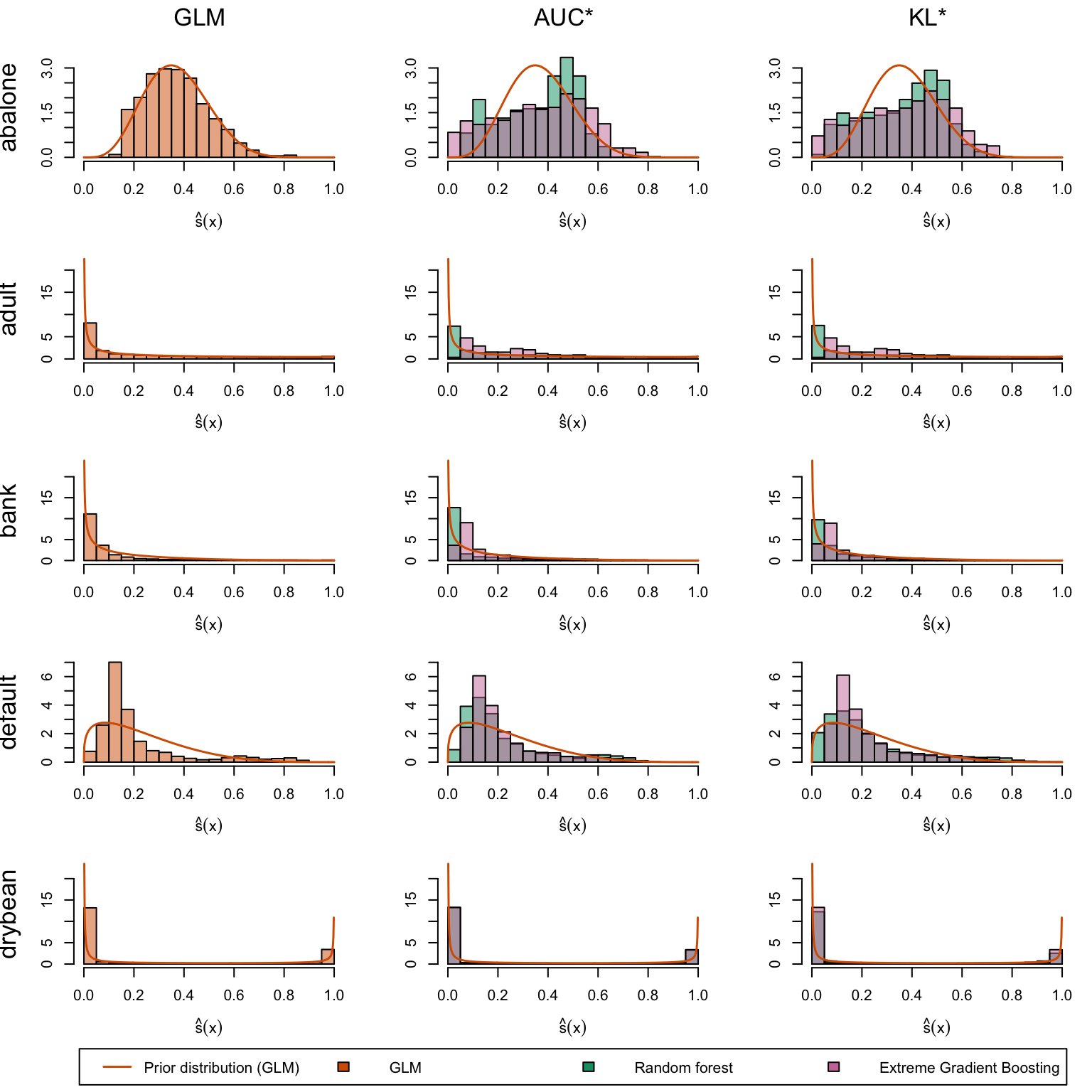
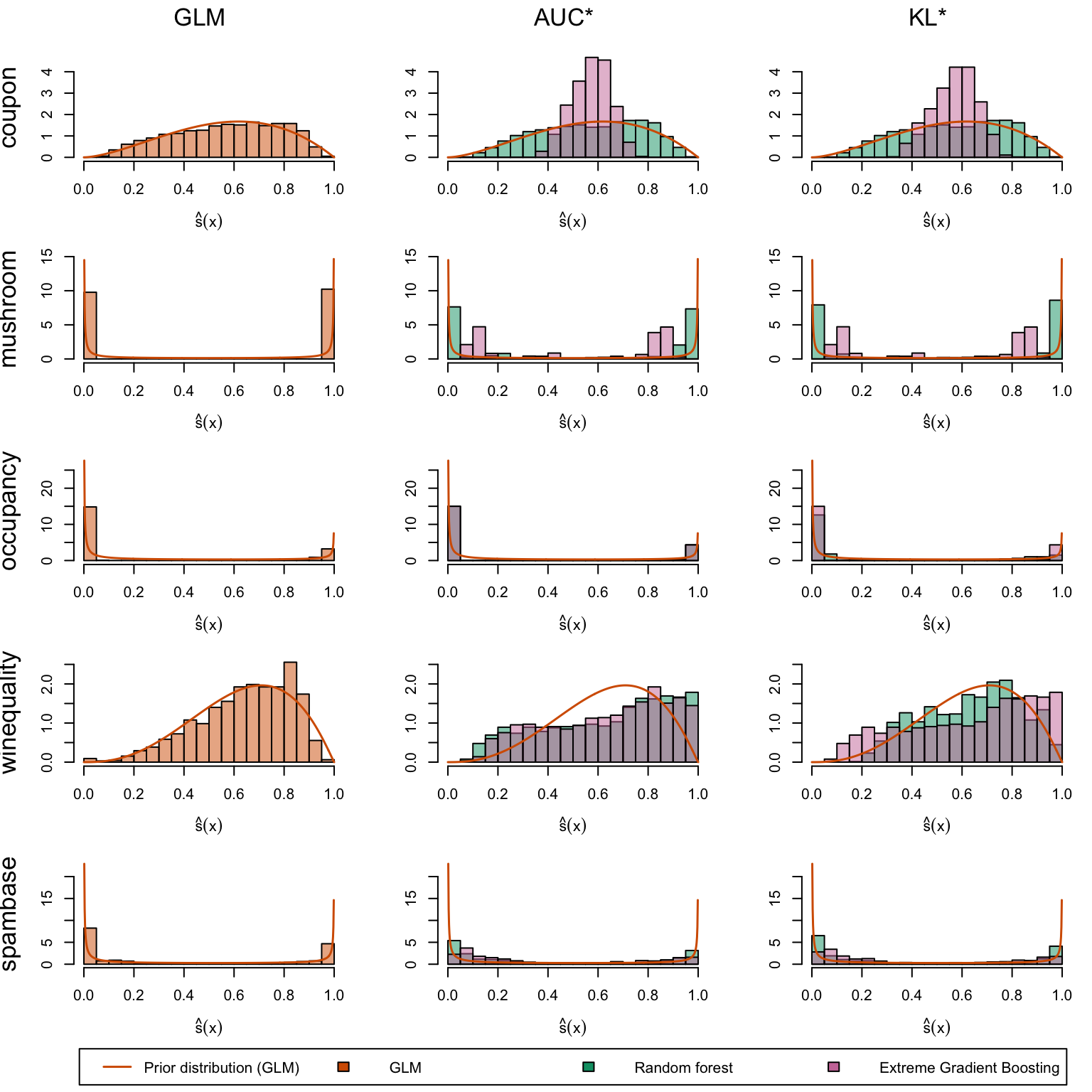
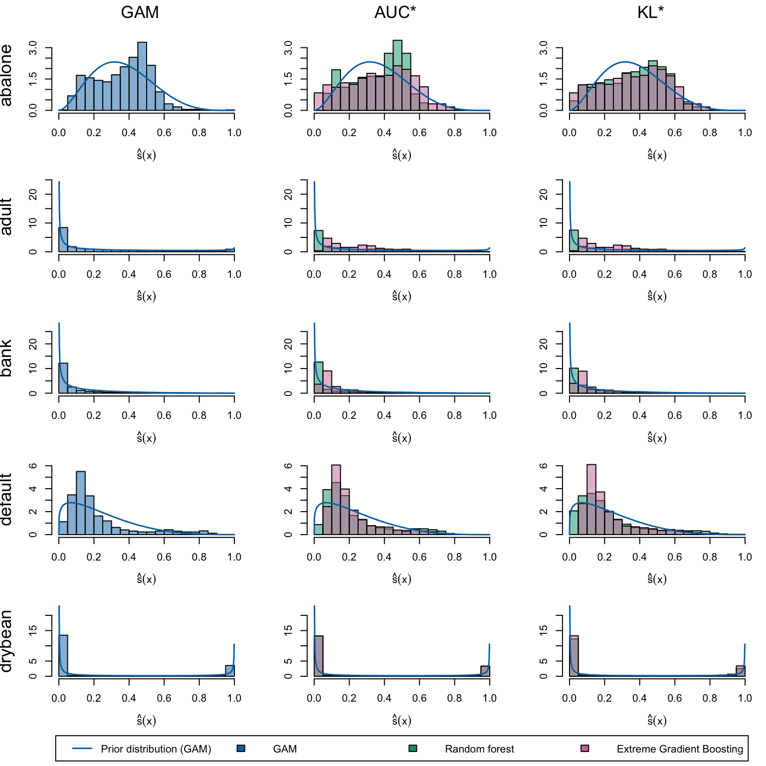
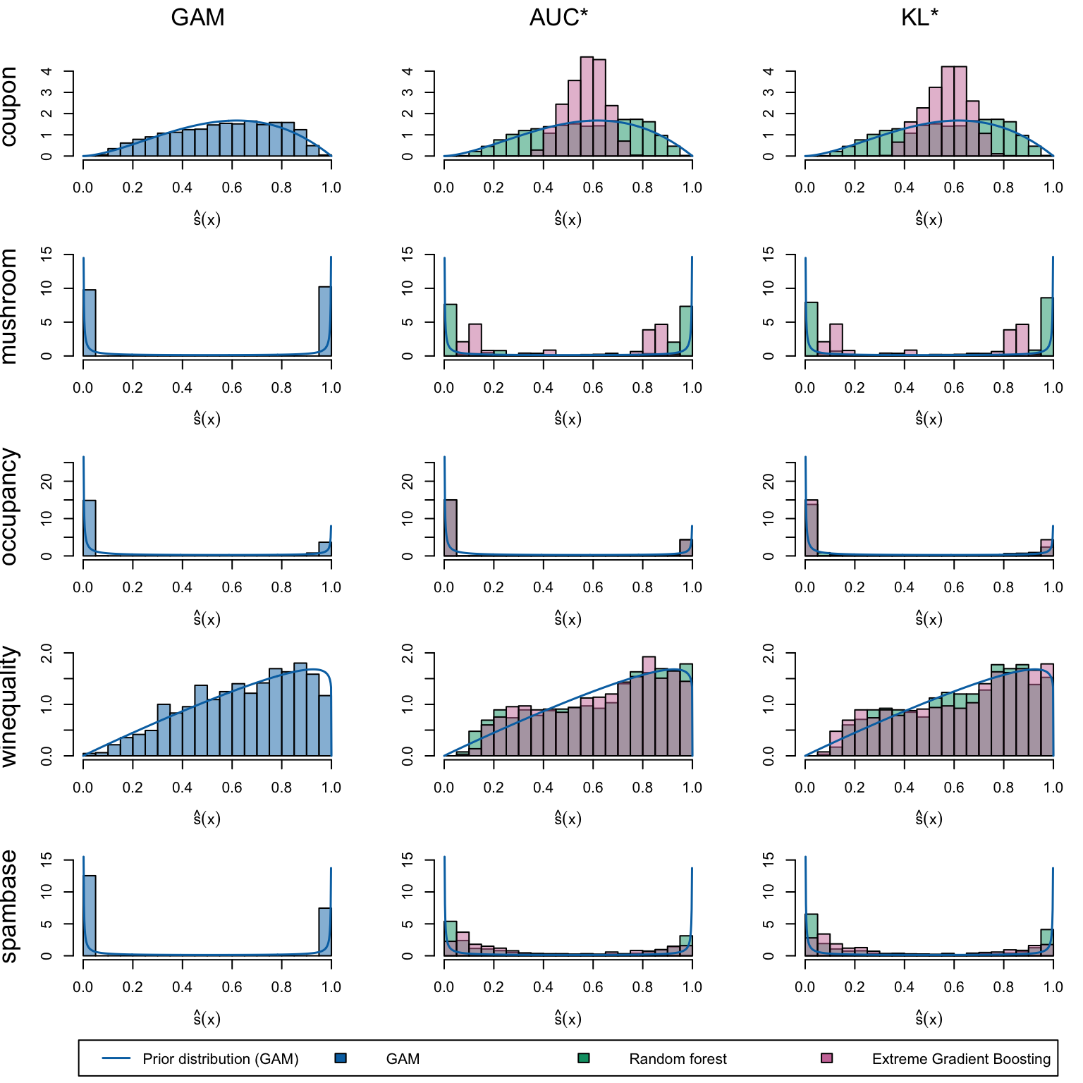
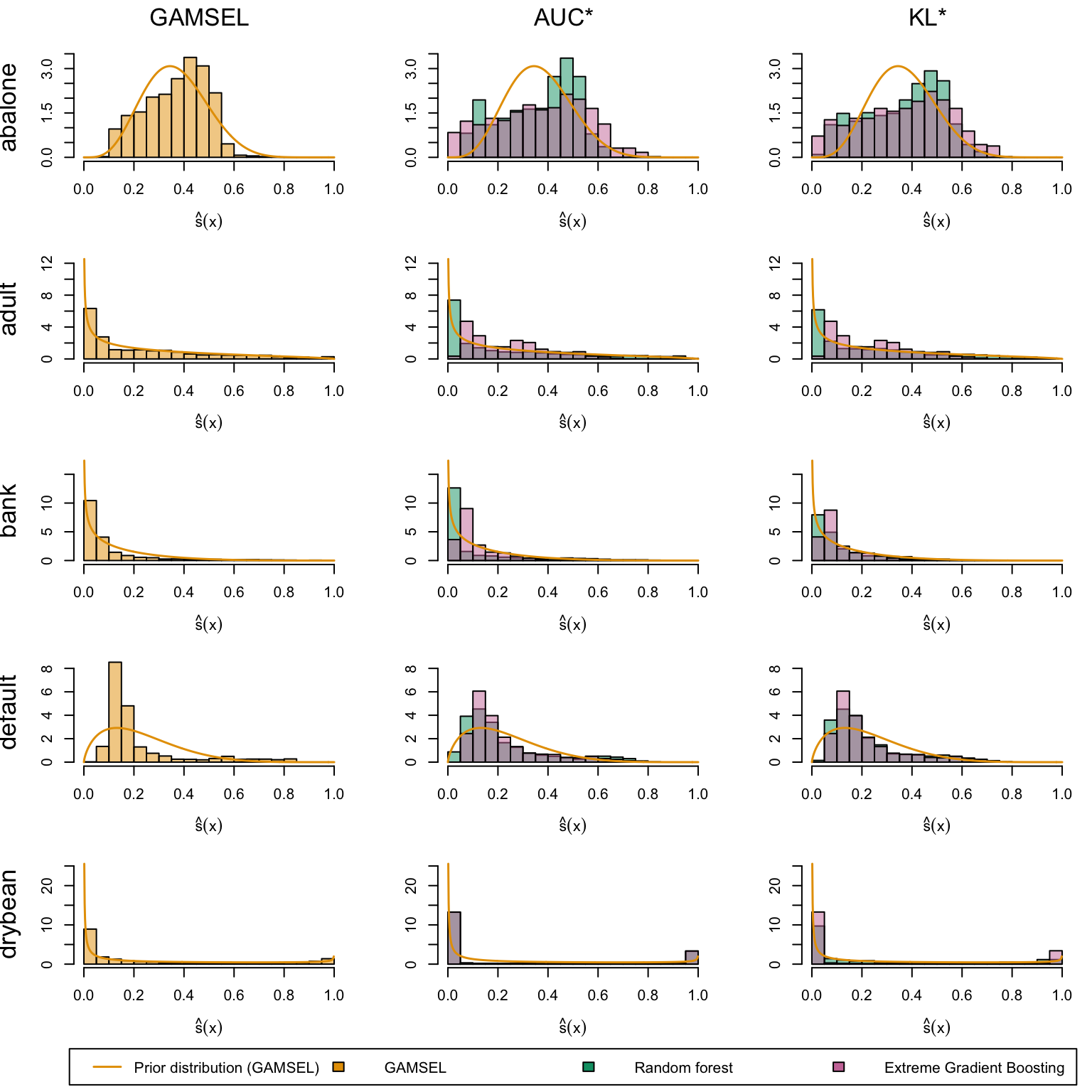
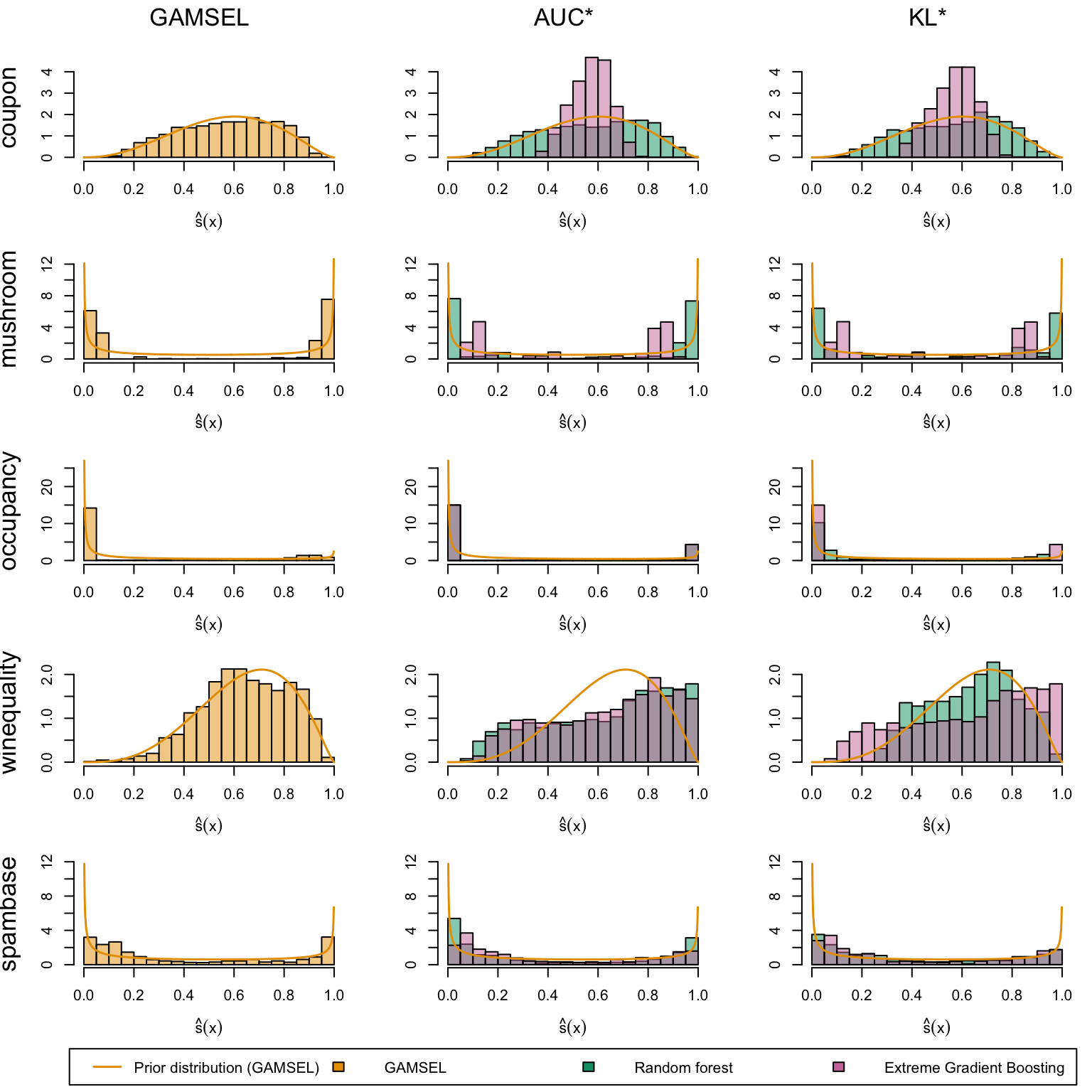
We define a (too long) function to create the plots. The left panel displays the score distribution estimated using a Generalized Linear Model. The middle panel presents scores estimated by the Random Forest and XGB models when maximizing the AUC. The right panel illustrates scores estimated by the Random Forest and XGB models when minimizing the KL divergence relative to the assumed probability distribution (a Beta distribution with shape parameters estimated from the scores in the left panel, see Chapter 14).

Display the too long plot function

print_plot <- function(prior_model, names) {
  prior_name <- prior_model_names |> filter(name == !!prior_model) |> 
    pull("label")
  col_titles <- c(prior_name, "AUC*", "KL*")
  layout(
    matrix(
      data = c(
        1:3,
        4:(length(names)*3+3),
        rep(length(names)*3+4, 3)
      ),
      ncol = 3, byrow = TRUE
    ), 
    heights = c(.5, rep(3, length(names)), .75)
  )
  
  # layout(matrix(c(1:6), ncol=3, byrow=T),heights = c(.5,3))
  par(mar = c(0, 4.1, 0, 2.1))
  for (i in 1:3) {
    plot(c(0, 1), c(0, 1), ann = F, bty = 'n', type = 'n', xaxt = 'n', yaxt = 'n')
    text(x = 0.5, y = 0.5, col_titles[i], cex = 1.6, col = "black")
  }
  
  colour_rf <- "#009E73"
  colour_xgb <- "#CC79A7"
  
  for (name in names) {
    # Get the histogram of scores estimated with the generalized linear model
    scores_prior <- priors[[name]][[str_c("scores_", prior_model)]]$scores_test
    priors_shapes <- priors[[name]][[str_c("mle_", prior_model)]]
    colour_prior <- prior_model_names |> filter(name == !!prior_model) |> 
      pull("colour")
    
    
    par(mar = c(4.1, 4.1, 1.1, 1.1))
    breaks <- seq(0, 1, by = .05)
    p_scores_prior <- hist(
      scores_prior, 
      breaks = breaks,
      plot = FALSE
    )
    val_u <- seq(0, 1, length = 651)
    dens_prior <- 
      dbeta(val_u, priors_shapes$estimate[1], priors_shapes$estimate[2])
    # Scores estimates with RF and XBG, maximizing AUC
    ind_score_hist_rf_auc <- 
      scores_ref_tibble |> 
      filter(model_interest == "max_auc", model_type == "rf", name == !!name) |> 
      pull("ind_list")
    ind_score_hist_xgb_auc <- 
      scores_ref_tibble |> 
      filter(model_interest == "max_auc", model_type == "xgb", name == !!name) |> 
      pull("ind_list")
    # Scores estimates with RF and XBG, minimizing KL
    ind_score_hist_rf_kl <- 
      scores_ref_tibble |> 
      filter(model_interest == !!prior_model, model_type == "rf", name == !!name) |> 
      pull("ind_list")
    ind_score_hist_xgb_kl <- 
      scores_ref_tibble |> 
      filter(model_interest == !!prior_model, model_type == "xgb", name == !!name) |> 
      pull("ind_list")
    
    p_max_auc_rf <- scores_hist[[ind_score_hist_rf_auc]]$test
    p_max_auc_xgb <- scores_hist[[ind_score_hist_xgb_auc]]$test
    p_min_kl_rf <- scores_hist[[ind_score_hist_rf_kl]]$test
    p_min_kl_xgb <- scores_hist[[ind_score_hist_xgb_kl]]$test
    
    y_lim <- c(
      range(dens_prior[!is.infinite(dens_prior)]),
      range(p_scores_prior$density),
      range(p_max_auc_rf$density),
      range(p_max_auc_xgb$density),
      range(p_min_kl_rf$density),
      range(p_min_kl_xgb$density)
    ) |> range()
    
    x_lab <- latex2exp::TeX("$\\hat{s}(x)$")
    plot(
      p_scores_prior,
      main = "",
      xlab = x_lab,
      ylab = "",
      freq = FALSE,
      ylim = y_lim,
      col = adjustcolor(colour_prior, alpha.f = .5)
    )
    lines(val_u, dens_prior, col = colour_prior, lwd = 1.5)
    # mtext(text = substitute(paste(bold(name))), side = 2, 
    #       line = 3, cex = 1, las = 0)
    mtext(text = name, side = 2, line = 3, cex = 1.1, las = 0)
    
    # Plot for max AUC
    plot(
      p_max_auc_rf,
      # main = "AUC*",
      main = "",
      xlab = x_lab,
      ylab = "",
      freq = FALSE,
      col = adjustcolor(colour_rf, alpha.f = .5),
      ylim = y_lim
    )
    plot(
      p_max_auc_xgb,
      add = TRUE,
      freq = FALSE,
      col = adjustcolor(colour_xgb, alpha.f = .5),
      y_lim = y_lim
    )
    lines(val_u, dens_prior, col = colour_prior, lwd = 1.5)
    
    # Plot for min KL
    plot(
      p_min_kl_rf,
      # main = "KL*",
      main = "",
      xlab = x_lab,
      ylab = "",
      freq = FALSE,
      col = adjustcolor(colour_rf, alpha.f = .5),
      ylim = y_lim
    )
    plot(
      p_min_kl_xgb,
      add = TRUE,
      freq = FALSE,
      col = adjustcolor(colour_xgb, alpha.f = .5),
      ylim = y_lim
    )
    lines(val_u, dens_prior, col = colour_prior, lwd = 1.5)
  }
  
  
  par(mar = c(0, 4.1, 0, 1.1))
  plot.new()
  legend(
    xpd = TRUE, ncol = 4,
    "center",
    lwd = c(1.5, rep(NA, 3)),
    col = c(colour_prior, rep(NA, 3)),
    fill = c(0, colour_prior, colour_rf, colour_xgb),
    legend = c(str_c("Prior distribution (", prior_name,")"), prior_name, "Random forest", "Extreme Gradient Boosting"),
    border=c(NA, "black","black","black")
  )
}

Datasets 1–5
Datasets 6–10

print_plot(prior_model = "glm", names = datasets$name[1:5])

Estimated scores on the first five datasets: GLM (left), models selected by AUC maximization (middle), and KL divergence minimization relative to prior assumptions (right).

print_plot(prior_model = "glm", names = datasets$name[6:10])

Estimated scores on the first last datasets: GLM (left), models selected by AUC maximization (middle), and KL divergence minimization relative to prior assumptions (right).

Datasets 1–5
Datasets 6–10

print_plot(prior_model = "gam", names = datasets$name[1:5])

Estimated scores on the first five datasets: GAM (left), models selected by AUC maximization (middle), and KL divergence minimization relative to prior assumptions (right).

print_plot(prior_model = "gam", names = datasets$name[6:10])

Datasets 1–5
Datasets 6–10

print_plot(prior_model = "gamsel", names = datasets$name[1:5])

Estimated scores on the first five datasets: GAMSEL (left), models selected by AUC maximization (middle), and KL divergence minimization relative to prior assumptions (right).

print_plot(prior_model = "gamsel", names = datasets$name[6:10])