This chapter illustrates the application of the method using real-world datasets. We train three models –a Generalized Linear Model (GLM), a Generalized Additive Model (GAM), and a Generalized Additive Model with model selection (GAMSEL)– on a binary variable to estimate the underlying event probabilities using available covariates. For each model, we derive scores from the test set and fit a Beta distribution via maximum likelihood estimation. This process yields three distinct priors for the true probability distribution of the event.
Code Availability
The functions for data preprocessing, model estimation, and Beta distribution fitting are stored in functions/real-data.R and will be used in subsequent chapters.
library(tidyverse)
── Attaching core tidyverse packages ──────────────────────── tidyverse 2.0.0 ──
✔ dplyr     1.1.4     ✔ readr     2.1.5
✔ forcats   1.0.0     ✔ stringr   1.5.1
✔ ggplot2   3.5.1     ✔ tibble    3.2.1
✔ lubridate 1.9.3     ✔ tidyr     1.3.1
✔ purrr     1.0.2
── Conflicts ────────────────────────────────────────── tidyverse_conflicts() ──
✖ dplyr::filter() masks stats::filter()
✖ dplyr::lag()    masks stats::lag()
ℹ Use the conflicted package (<http://conflicted.r-lib.org/>) to force all conflicts to become errors
library(gam)
Loading required package: splines
Loading required package: foreach

Attaching package: 'foreach'

The following objects are masked from 'package:purrr':

    accumulate, when

Loaded gam 1.22-3
library(gamsel)
Loaded gamsel 1.8-4
# Colours for train/testcolour_samples <-c("Train"="#0072B2","Test"="#D55E00")
13.1 Raw Data
To illustrate the process, we use the spambase dataset (available on UCI Machine Learning Repository). The dataset contains 4,601 rows. The target variable, is_spam will be explained using the 57 continuous predictors.
The dataset can be downloaded as follows:
if (!dir.exists("data")) dir.create("data")download.file(url ="https://archive.ics.uci.edu/static/public/94/spambase.zip", destfile ="data/spambase.zip")
The names of the columns are given in the spambase.names file in that archive.
# This chunk is not runinfo_data <-scan(unz("data/spambase.zip", "spambase.names"), what ="character", sep ="\n")# Print the names for this dataset (not very convenient...)str_extract(info_data[31:length(info_data)], "^(.*):") |>str_remove(":$") |> (\(.x) str_c('"', .x, '",'))() |>cat()
Rows: 4601 Columns: 58
── Column specification ────────────────────────────────────────────────────────
Delimiter: ","
dbl (58): word_freq_make, word_freq_address, word_freq_all, word_freq_3d, wo...

ℹ Use `spec()` to retrieve the full column specification for this data.
ℹ Specify the column types or set `show_col_types = FALSE` to quiet this message.
The target variable is is_spam.
target_name <-"is_spam"
13.2 Data Pre-processing
We define two functions to pre-process the data. The first one, split_train_test() simply split the dataset into two subsets: one for training the models (train) and another one for testing the models (test).
#' Split dataset into train and test set#'#' @param data dataset#' @param prop_train proportion in the train test (default to .8)#' @param seed desired seed (default to `NULL`)#'#' @returns a list with two elements: the train set, the test setsplit_train_test <-function(data,prop_train = .8,seed =NULL) {if (!is.null(seed)) set.seed(seed) size_train <-round(prop_train *nrow(data)) ind_sample <-sample(1:nrow(data), replace =FALSE, size = size_train)list(train = data |> dplyr::slice(ind_sample),test = data |> dplyr::slice(-ind_sample) )}
With the current dataset:
data <-split_train_test(data = dataset, prop_train = .8, seed =1234)names(data)
[1] "train" "test"
Some of the models we use need the data to be numerical. We thus build a function, encode_dataset() that transforms the categorical columns into sets of dummy variables. For each categorical variable, we remove one of the levels to avoid colinearity in the predictor matrix. This step is made using the convenient functions from the {recipes} package. In addition, the spline function from the {gam} package does not support variables with names that do not respect the R naming conventions. We thus rename all the variables and keep track of the changes.
The encode_dataset() returns a list with five elements:
train: the train set where categorical variables have been transformed into dummy variables
test: the test set where categorical variables have been transformed into dummy variables
initial_covariate_names: vector of names of all explanatory variables
categ_names: vector of new names of categorical variables (if any)
covariate_names: vector of new names of all explanatory variables (including categorigal ones).
#' One-hot encoding, and renaming variables to avoid naming that do not respect#' r old naming conventions#'#' @param data_train train set#' @param data_test test set#' @param target_name name of the target (response) variable#' @param intercept should a column for an intercept be added? Default to#' `FALSE`#'#' @returns list with five elements:#' - `train`: train set#' - `test`: test set#' - `initial_covariate_names`: vector of names of all explanatory variables#' - `categ_names`: vector of new names of categorical variables (if any)#' - `covariate_names`: vector of new names of all explanatory variables (including#' categorical ones).encode_dataset <-function(data_train, data_test, target_name,intercept =FALSE) { col_names <-colnames(data_train) col_names_covariates <- col_names[-which(col_names == target_name)] new_names_covariates <-str_c("X_", 1:length(col_names_covariates)) data_train <- data_train |>rename_with(.cols =all_of(col_names_covariates), .fn =~new_names_covariates) data_test <- data_test |>rename_with(.cols =all_of(col_names_covariates), .fn =~new_names_covariates) data_rec <- recipes::recipe(formula(str_c(target_name, " ~ .")),data = data_train ) ref_cell <- data_rec |> recipes::step_dummy( recipes::all_nominal(), -recipes::all_outcomes(),one_hot =TRUE ) |> recipes::prep(training = data_train) X_train_dmy <- recipes::bake(ref_cell, new_data = data_train) X_test_dmy <- recipes::bake(ref_cell, new_data = data_test)# Identify categorical variables# Bake the recipe to apply the transformation df_transformed <- recipes::bake(ref_cell, new_data =NULL)# Get the names of the transformed data new_names <-names(X_train_dmy) original_vars <-names(data_train) categ_names <-setdiff(new_names, original_vars) covariate_names <-colnames(X_train_dmy) covariate_names <- covariate_names[!covariate_names == target_name] categ_names <- categ_names[!categ_names == target_name]list(train = X_train_dmy,test = X_test_dmy,initial_covariate_names = col_names_covariates,categ_names = categ_names,covariate_names = covariate_names )}
Let us use the encode_dataset() function to rename the columns here. As there is no categorical variable among the predictors, no dummy variable will be created.
Let us estimate the probability that the event occurs (the email is a spam) using a Generalized Linear Model with a logistic link function.
We first build the formula:
form <-str_c(target_name, "~.") |>as.formula()
Then, we fit the model:
fit <-glm(form, data = data_dmy$train, family ="binomial")
Lastly, we can get the predicted scores:
scores_train <-predict(fit, newdata = data_dmy$train, type ="response")scores_test <-predict(fit, newdata = data_dmy$test, type ="response")
We encompass these steps in a helper function:
#' Train a GLM-logistic model#'#' @param data_train train set#' @param data_test test set#' @param target_name name of the target (response) variable#' @param return_model if TRUE, the estimated model is returned#'#' @returns list with estimated scores on train set (`scores_train`) and on#' test set (`scores_test`)train_glm <-function(data_train, data_test, target_name,return_model =FALSE) {# Encode dataset so that categorical variables become dummy variables data_dmy <-encode_dataset(data_train = data_train,data_test = data_test,target_name = target_name,intercept =FALSE )# Formula for the model form <-str_c(target_name, "~.") |>as.formula()# Estimation fit <-glm(form, data = data_dmy$train, family ="binomial")# Scores on train and test set scores_train <-predict(fit, newdata = data_dmy$train, type ="response") scores_test <-predict(fit, newdata = data_dmy$test, type ="response")if (return_model ==TRUE) { res <-list(scores_train = scores_train, scores_test = scores_test, fit = fit) } else {list(scores_train = scores_train, scores_test = scores_test, fit =NULL) }}
This function can then be used in a very simple way:
Warning: glm.fit: fitted probabilities numerically 0 or 1 occurred
13.3.2 GAM
We then estimate the probability that the event occurs (the email is a spam) using a Generalized Additive Model.
We first build the formula. Here, this is a tiny bit more complex than with the GLM. The model will contain smooth terms (for numerical variables) and linear terms (for categorical variables which, if present in the data, were encoded as dummy variables).
Then, we count the number of unique values for each variable. This step ensures that the smoothing parameter of the spline function applied to numerical variables is not larger than the number of unique values. We arbitrarily set the smoothing parameter to 6. But if the number of unique values for a variable is lower than this, then we use the number of unique values minus 1 as the smoothing parameter for that variable.
Then, we need to make sure that all variables obtained after using the encode_dataset() function are coded as numeric: the estimation function from {gamsel} does not allow integer variables.
Then we need to build the formula. As for the GAM, this is a bit more complex that with the GLM. We need to create a vector that gives the maximum spline basis function to use for each variable. For dummy variables, this needs to be set to 1. For other variables, let us use either 6 or the minimum number of distinct values minus 1.
Then, we fit the model. The penalty parameter \(\lambda\) is selected by 10-fold cross validation in a first step:
gamsel_cv <- gamsel::cv.gamsel(x =as.data.frame(X_dmy_train), y = y_train, family ="binomial",degrees = deg)
We use the value of lambda which gives the minimum cross validation metric. Note that we could also use the largest value of lambda such that the error is within 1 standard error of the minimum (using lambda = gamsel_cv$lambda.1se):
gamsel_out <-gamsel(x =as.data.frame(X_dmy_train), y = y_train, family ="binomial",degrees = deg,lambda = gamsel_cv$lambda.min)
Lastly, we can get the predicted scores:
scores_train <-predict( gamsel_out, newdata =as.data.frame(X_dmy_train), type ="response")[, 1] scores_test <-predict( gamsel_out, newdata =as.data.frame(X_dmy_test), type ="response")[, 1]
We encompass these steps in a helper function:
#' Train a GAMSEL model#'#' @param data_train train set#' @param data_test test set#' @param target_name name of the target (response) variable#' @param degrees degree for the splines#' @param return_model if TRUE, the estimated model is returned#'#' @returns list with estimated scores on train set (`scores_train`) and on#' test set (`scores_test`)train_gamsel <-function(data_train, data_test, target_name,degrees =6,return_model =FALSE) {# Encode dataset so that categorical variables become dummy variables data_dmy <-encode_dataset(data_train = data_train,data_test = data_test,target_name = target_name,intercept =FALSE )# Estimation X_dmy_train <- data_dmy$train |> dplyr::select(-!!target_name) X_dmy_train <- X_dmy_train |>mutate(across(everything(), as.numeric)) X_dmy_test <- data_dmy$test |> dplyr::select(-!!target_name) X_dmy_test <- X_dmy_test |>mutate(across(everything(), as.numeric)) y_train <- data_dmy$train |> dplyr::pull(!!target_name) y_test <- data_dmy$test |> dplyr::pull(!!target_name) deg <-rep(NA, ncol(X_dmy_train)) col_names_X <-colnames(X_dmy_train) nb_val <-map_dbl( col_names_X, ~X_dmy_train |>pull(.x) |>unique() |>length() )for (i_var_name in1:ncol(X_dmy_train)) { var_name <- col_names_X[i_var_name]if (var_name %in% data_dmy$categ_names) { deg[i_var_name] <-1 } else { deg[i_var_name] <-min(nb_val[i_var_name]-1, degrees) } } gamsel_cv <- gamsel::cv.gamsel(x =as.data.frame(X_dmy_train), y = y_train, family ="binomial",degrees = deg ) gamsel_out <- gamsel::gamsel(x =as.data.frame(X_dmy_train), y = y_train, family ="binomial",degrees = deg,lambda = gamsel_cv$lambda.min )# Scores on train and test set scores_train <-predict( gamsel_out, newdata =as.data.frame(X_dmy_train), type ="response")[, 1] scores_test <-predict( gamsel_out, newdata =as.data.frame(X_dmy_test), type ="response")[, 1]if (return_model ==TRUE) { res <-list(scores_train = scores_train,scores_test = scores_test,fit = fit) } else {list(scores_train = scores_train, scores_test = scores_test, fit =NULL) }}
This function can then be used in a very simple way:
Once the scores from the models have been estimated, we fit a Beta distribution to them. This will provide a prior distribution of the true probabilities in the exercise.
To avoid crashing the ML estimation of the two parameters of the Beta distribution, let us make sure that any score is in \((0,1)\) and not exactly equal to 0 or 1.
To estimate the two parameters of the Beta distribution, we define a small function, fit_beta_scores() that calls the fitdistr() function from {MASS}.
#' Maximum-likelihood fitting of Beta distribution on scores#'#' @param scores vector of estimated scores#' @param shape1 non-negative first parameter of the Beta distribution#' @param shape1 non-negative second parameter of the Beta distribution#'#' @returns An object of class `fitdistr`, a list with four components#' (see: MASS::fitdistr())#' - `estimate`: the parameter estimates#' - `sd`: the estimated standard errors#' - `vcov`: the estimated variance-covariance matrix#' - `loglik`: the log-likelihoodfit_beta_scores <-function(scores, shape1 =1, shape2 =1) {# Fit a beta distribution mle_fit <- MASS::fitdistr( scores, "beta", start =list(shape1 =1, shape2 =1) ) mle_fit}
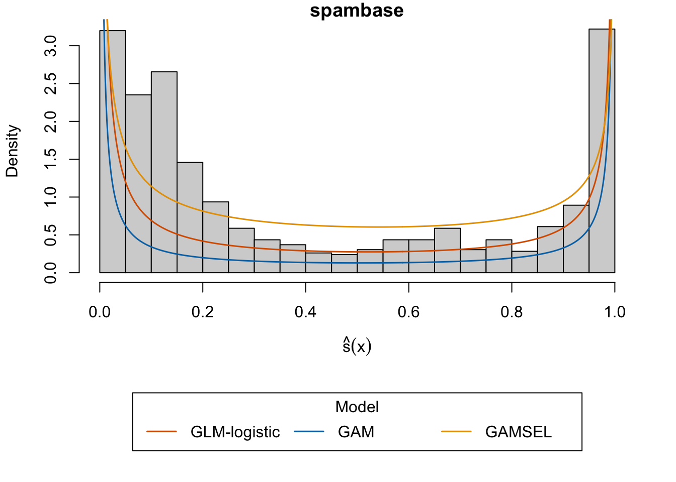
Let us plot the distribution of the scores obtained with the GAMSEL model. On top of the graph, we draw the density of the Beta distribution with the parameters estimated for each model.
Code
val_u <-seq(0, 1, length =651)layout(mat =matrix(1:2), heights =c(3,1))# Histogram of scores obtained with the GAMSEL, on test setpar(mar =c(4.1, 4.1, 1, 2.1))hist( scores_gamsel$scores_test,breaks =seq(0, 1, by = .05), probability =TRUE,main ="spambase", xlab = latex2exp::TeX("$\\hat{s}(x)$"))# Beta dist. estimated using the scores from the GLMlines( val_u,dbeta(val_u, mle_glm$estimate[1], mle_glm$estimate[2]),col ="#D55E00",lwd =1.5)# Beta dist. estimated using the scores from the GAMlines( val_u,dbeta(val_u, mle_gam$estimate[1], mle_gam$estimate[2]),col ="#0072B2",lwd =1.5)# Beta dist. estimated using the scores from the GAMlines( val_u,dbeta(val_u, mle_gamsel$estimate[1], mle_gamsel$estimate[2]),col ="#E69F00",lwd =1.5)par(mar =c(0, 4.1, 0, 2.1))plot.new()legend(xpd =TRUE, ncol =3,"center",title ="Model",lwd =1.5,col =c("#D55E00", "#0072B2", "#E69F00"),legend =c("GLM-logistic", "GAM", "GAMSEL"))
Figure 13.1: Distribution of estimated probabilities by the GAMSEL model and Beta distribution fitted to the scores of each of the three models.
13.5 Wrapper Functions
For convenience, we build a wrapper function, get_beta_fit() that takes a dataset as an input, the name of the target variable and possibly a seet. From these arguments, the function splits the dataset into a training and a test set. It then fits the models, and fit a Beta distribution on the scores estimated in the test set. This function returns a list with 6 elements: the first three are the estimated scores of the three models, the last three are the parameters of the Beta distribution estimated using the scores of each model.
Function get_beta_fit()
#' Estimation of a GLM-logistic, a GAM and a GAMSEL model on a classification#' task. Then, on estimated scores from the test set, fits a Beta distribution.#'#' @param dataset dataset with response variable and predictors#' @param target_name name of the target (response) variable#' @param seed desired seed (default to `NULL`)#'#' @returns A list with the following elements:#' - `scores_glm`: scores on train and test set (in a list) from the GLM#' - `scores_gam`: scores on train and test set (in a list) from the GAM#' - `scores_gamsel`: scores on train and test set (in a list) from the GAMSEL#' - `mle_glm`: An object of class "fitdistr" for the GLM model#' (see fit_beta_scores())#' - `mle_gamsel`: An object of class "fitdistr" for the GAM model#' (see fit_beta_scores())#' - `mle_gamsel`: An object of class "fitdistr" for the GAMSEL model#' (see fit_beta_scores())get_beta_fit <-function(dataset, target_name,seed =NULL) {# Split data into train/test data <-split_train_test(data = dataset, prop_train = .8, seed = seed)# Train a GLM-logistic model scores_glm <-train_glm(data_train = data$train, data_test = data$test, target_name = target_name )# Train a GAM model scores_gam <-train_gam(data_train = data$train, data_test = data$test, target_name = target_name,spline_df =6 )# Train a GAMSEL model scores_gamsel <-train_gamsel(data_train = data$train, data_test = data$test, target_name = target_name,degrees =6 )# Add a little noise to the estimated scores to avoid being in [0,1] and be# in (0,1) instead. x_glm <- (scores_glm$scores_test * (1-1e-6)) +1e-6/2 x_gam <- (scores_gam$scores_test * (1-1e-6)) +1e-6/2 x_gamsel <- (scores_gamsel$scores_test * (1-1e-6)) +1e-6/2# Fit a Beta distribution on these scores mle_gam <-fit_beta_scores(scores = x_gam) mle_glm <-fit_beta_scores(scores = x_glm) mle_gamsel <-fit_beta_scores(scores = x_gamsel)list(scores_glm = scores_glm,scores_gam = scores_gam,scores_gamsel = scores_gamsel,mle_glm = mle_glm,mle_gam = mle_gam,mle_gamsel = mle_gamsel )}
We also define a function, plot_hist_scores_beta() to plot the distribution of scores obtained with the GAMSEL model and the density functions of the three Beta distributions whose parameters were estimated based on the scores of the three models.
Function plot_hist_scores_beta()
#' Plots the histogram of scores estimated with GAMSEL#' add densities of Beta distribution for whith the parameters have been#' estimated using scores from the GLM, the GAM, or the GAMSEL model#'#' @param fit_resul results obtained from get_beta_fit()#' @param title title of the graph (e.g.: dataset name)plot_hist_scores_beta <-function(fit_resul, title =NULL) { val_u <-seq(0, 1, length =651)layout(mat =matrix(1:2), heights =c(3,1)) dbeta_val <-vector(mode ="list", length =3)for (i_type in1:3) { type <-c("mle_glm", "mle_gam", "mle_gamsel")[i_type] dbeta_val[[i_type]] <-dbeta( val_u, fit_resul[[type]]$estimate[1], fit_resul[[type]]$estimate[2] ) } y_lim <-c(0,map(dbeta_val,~range(.x[!is.infinite(.x)], na.rm =TRUE)) |>unlist() |>max(na.rm =TRUE) )# Histogram of scores obtained with the GAMSEL, on test setpar(mar =c(4.1, 4.1, 1, 2.1))hist( fit_resul$scores_gamsel$scores_test,breaks =seq(0, 1, by = .05), probability =TRUE,main = title, xlab = latex2exp::TeX("$\\hat{s}(x)$"),ylim = y_lim ) legend_name <-c("GLM-logistic", "GAM", "GAMSEL") colours <-c("mle_glm"="#D55E00","mle_gam"="#0072B2","mle_gamsel"="#E69F00" )for (i_type in1:3) { type <-c("mle_glm", "mle_gam", "mle_gamsel")[i_type]lines( val_u, dbeta_val[[i_type]],col = colours[i_type],lwd =1.5 ) }par(mar =c(0, 4.1, 0, 2.1))plot.new()legend(xpd =TRUE, ncol =3,"center",title ="Model",lwd =1.5,col = colours,legend = legend_name )}