5 Decision Trees

Note

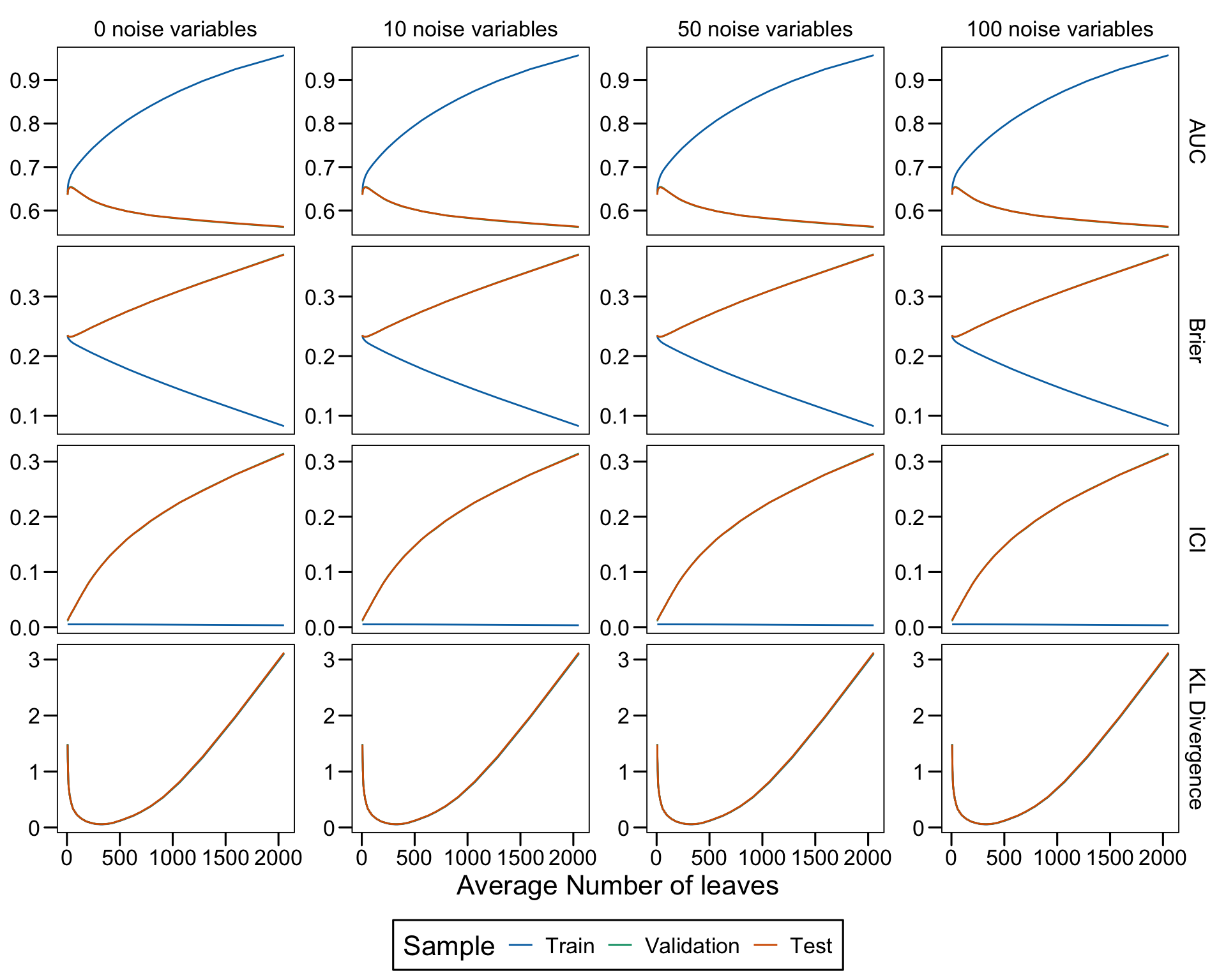
This chapter investigates how scores returned by a decision tree are impacted by the tree complexity. We vary the minimal number of observation in terminal leaves to obtain trees with varying number of leaves. In the resulting estimated trees, we look at the scores.

library(tidyverse)

── Attaching core tidyverse packages ──────────────────────── tidyverse 2.0.0 ──
✔ dplyr     1.1.4     ✔ readr     2.1.5
✔ forcats   1.0.0     ✔ stringr   1.5.1
✔ ggplot2   3.5.1     ✔ tibble    3.2.1
✔ lubridate 1.9.3     ✔ tidyr     1.3.1
✔ purrr     1.0.2     
── Conflicts ────────────────────────────────────────── tidyverse_conflicts() ──
✖ dplyr::filter() masks stats::filter()
✖ dplyr::lag()    masks stats::lag()
ℹ Use the conflicted package (<http://conflicted.r-lib.org/>) to force all conflicts to become errors

library(ggh4x)


Attaching package: 'ggh4x'

The following object is masked from 'package:ggplot2':

    guide_axis_logticks

library(rpart)
library(locfit)

locfit 1.5-9.9   2024-03-01

Attaching package: 'locfit'

The following object is masked from 'package:purrr':

    none

library(philentropy)
# remotes::install_github("gweissman/gmish")

# Colours for train/test
colour_samples <- c(
  "Train" = "#0072B2",
  "Validation" = "#009E73",
  "Test" = "#D55E00"
)

definition of the theme_paper() function (for ggplot2 graphs)

#' Theme for ggplot2
#'
#' @param ... arguments passed to the theme function
#' @export
#' @importFrom ggplot2 element_rect element_text element_blank element_line unit
#'   rel
theme_paper <- function (...) {
  ggthemes::theme_base() +
    theme(
      plot.background = element_blank(),
      legend.background = element_rect(
        fill = "transparent", linetype="solid", colour ="black"),
      legend.position = "bottom",
      legend.direction = "horizontal",
      legend.box = "horizontal",
      legend.key = element_blank()
    )
}

5.1 Data

We generate data using the first 12 scenarios from Ojeda et al. (2023) and an additional set of 4 scenarios in which the true probability does not depend on the predictors in a linear way (see Chapter 4).

source("functions/data-ojeda.R")
library(ks)
source("functions/subsample_target_distribution.R")

When we simulate a dataset, we draw the following number of observations:

nb_obs <- 10000

Definition of the 16 scenarios

# Coefficients beta
coefficients <- list(
  # First category (baseline, 2 covariates)
  c(0.5, 1),  # scenario 1, 0 noise variable
  c(0.5, 1),  # scenario 2, 10 noise variables
  c(0.5, 1),  # scenario 3, 50 noise variables
  c(0.5, 1),  # scenario 4, 100 noise variables
  # Second category (same as baseline, with lower number of 1s)
  c(0.5, 1),  # scenario 5, 0 noise variable
  c(0.5, 1),  # scenario 6, 10 noise variables
  c(0.5, 1),  # scenario 7, 50 noise variables
  c(0.5, 1),  # scenario 8, 100 noise variables
  # Third category (same as baseline but with 5 num. and 5 categ. covariates)
  c(0.1, 0.2, 0.3, 0.4, 0.5, 0.01, 0.02, 0.03, 0.04, 0.05),
  c(0.1, 0.2, 0.3, 0.4, 0.5, 0.01, 0.02, 0.03, 0.04, 0.05),
  c(0.1, 0.2, 0.3, 0.4, 0.5, 0.01, 0.02, 0.03, 0.04, 0.05),
  c(0.1, 0.2, 0.3, 0.4, 0.5, 0.01, 0.02, 0.03, 0.04, 0.05),
  # Fourth category (nonlinear predictor, 3 covariates)
  c(0.5, 1, .3),  # scenario 5, 0 noise variable
  c(0.5, 1, .3),  # scenario 6, 10 noise variables
  c(0.5, 1, .3),  # scenario 7, 50 noise variables
  c(0.5, 1, .3)  # scenario 8, 100 noise variables
)

# Mean parameter for the normal distribution to draw from to draw num covariates
mean_num <- list(
  # First category (baseline, 2 covariates)
  rep(0, 2),  # scenario 1, 0 noise variable
  rep(0, 2),  # scenario 2, 10 noise variables
  rep(0, 2),  # scenario 3, 50 noise variables
  rep(0, 2),  # scenario 4, 100 noise variables
  # Second category (same as baseline, with lower number of 1s)
  rep(0, 2),  # scenario 5, 0 noise variable
  rep(0, 2),  # scenario 6, 10 noise variables
  rep(0, 2),  # scenario 7, 50 noise variables
  rep(0, 2),  # scenario 8, 100 noise variables
  # Third category (same as baseline but with 5 num. and 5 categ. covariates)
  rep(0, 5),
  rep(0, 5),
  rep(0, 5),
  rep(0, 5),
  # Fourth category (nonlinear predictor, 3 covariates)
  rep(0, 3),
  rep(0, 3),
  rep(0, 3),
  rep(0, 3)
)
# Sd parameter for the normal distribution to draw from to draw num covariates
sd_num <- list(
  # First category (baseline, 2 covariates)
  rep(1, 2),  # scenario 1, 0 noise variable
  rep(1, 2),  # scenario 2, 10 noise variables
  rep(1, 2),  # scenario 3, 50 noise variables
  rep(1, 2),  # scenario 4, 100 noise variables
  # Second category (same as baseline, with lower number of 1s)
  rep(1, 2),  # scenario 5, 0 noise variable
  rep(1, 2),  # scenario 6, 10 noise variables
  rep(1, 2),  # scenario 7, 50 noise variables
  rep(1, 2),  # scenario 8, 100 noise variables
  # Third category (same as baseline but with 5 num. and 5 categ. covariates)
  rep(1, 5),
  rep(1, 5),
  rep(1, 5),
  rep(1, 5),
  # Fourth category (nonlinear predictor, 3 covariates)
  rep(1, 3),
  rep(1, 3),
  rep(1, 3),
  rep(1, 3)
)

params_df <- tibble(
  scenario = 1:16,
  coefficients = coefficients,
  n_num = c(rep(2, 8), rep(5, 4), rep(3, 4)),
  add_categ = c(rep(FALSE, 8), rep(TRUE, 4), rep(FALSE, 4)),
  n_noise = rep(c(0, 10, 50, 100), 4),
  mean_num = mean_num,
  sd_num = sd_num,
  size_train = rep(nb_obs, 16),
  size_valid = rep(nb_obs, 16),
  size_test = rep(nb_obs, 16),
  transform_probs = c(rep(FALSE, 4), rep(TRUE, 4), rep(FALSE, 4), rep(FALSE, 4)),
  linear_predictor = c(rep(TRUE, 12), rep(FALSE, 4)),
  seed = 202105
)
rm(coefficients, mean_num, sd_num)

5.2 Metrics

We load the functions from Chapter 3 to compute performance, calibration and divergence metrics.

source("functions/metrics.R")

5.3 Simulations Setup

For each scenario, we will grow a tree to predict the binary outcome using all the available variables in the simulated dataset. We train regression trees here, as we are interested in the resulting scores, not by the class given by a majority vote.

The desired number of replications for each scenario needs to be set:

repns_vector <- 1:100

To obtain trees with varying number of leaves, we make the min_bucket parameter vary. This parameter defines the minimal number of observation in a terminal leaf node. A split is not performed if at least one of the resulting children leaves do not contain at least min_bucket observations. In addition, a split will not be attempted if the number of observation in the current node is lower than three times min_bucket.

For each scenario (i.e., different data generating process), we consider 100 replications: we draw 100 samples from the data generating process associated with the scenario.

5.3.1 Estimation Function

We define the simul_tree() function to make a single replication of the simulations.

Function simul_tree()

#' Train a tree and compute performance, calibration, and dispersion metrics.
#' 
#' @param prune should the tree be pruned?
#' @param min_bucket minimal number of observations in terminal nodes
#' @param type either `"regression"` for regression tree or `"classification"`
#'  for classification tree
#' @param simu_data simulated data obtained with `simulate_data_wrapper()`
#' @param ind numerical ID of the simulation in the grid: different from the 
#'  seed ID)
simul_tree <- function(prune = c(TRUE, FALSE),
                       min_bucket,
                       type = c("regression", "classification"),
                       simu_data,
                       ind) {

  tb_train <- simu_data$data$train |> rename(d = y)
  tb_valid <- simu_data$data$valid |> rename(d = y)
  tb_test <- simu_data$data$test |> rename(d = y)

  true_prob <-
    list(
      train = simu_data$data$probs_train,
      valid = simu_data$data$probs_valid,
      test = simu_data$data$probs_test
    )

  # Estimation----
  if (type == "regression") {
    estim_tree <- rpart(
      d ~ x1 + x2, data = tb_train,
      method = "anova",
      minsplit = min_bucket * 3,
      minbucket = min_bucket,
      cp = 0
    )
  } else {
    estim_tree <- rpart(
      d ~ x1 + x2, data = tb_train,
      method = "class",
      minsplit = min_bucket * 3,
      minbucket = min_bucket,
      cp = 0
    )
  }
  if (prune == TRUE) {
    ind_min_cp <- which.min(estim_tree$cptable[,"xerror"])
    min_cp <- estim_tree$cptable[ind_min_cp, "CP"]
    estim_tree <- prune(estim_tree, cp = min_cp)
  }

  nb_leaves <- sum(estim_tree$frame$var=="<leaf>")
  depth <- max(rpart:::tree.depth(as.numeric(rownames(estim_tree$frame))))

  # Raw Scores----
  # Predicted scores
  if (type == "regression") {
    scores_train <- predict(estim_tree, newdata = tb_train)
    scores_valid <- predict(estim_tree, newdata = tb_valid)
    scores_test <- predict(estim_tree, newdata = tb_test)
  } else {
    scores_train <- predict(estim_tree, newdata = tb_train)[,"1"]
    scores_valid <- predict(estim_tree, newdata = tb_valid)[,"1"]
    scores_test <- predict(estim_tree, newdata = tb_test)[,"1"]
  }

  # Histogram of scores
  breaks <- seq(0, 1, by = .05)
  scores_train_hist <- hist(scores_train, breaks = breaks, plot = FALSE)
  scores_valid_hist <- hist(scores_valid, breaks = breaks, plot = FALSE)
  scores_test_hist <- hist(scores_test, breaks = breaks, plot = FALSE)
  scores_hist <- list(
    train = scores_train_hist,
    valid = scores_valid_hist,
    test = scores_test_hist
  )

  # Estimation of P(q1 < score < q2)
  proq_scores_train <- map(
    c(.1, .2, .3, .4),
    ~prop_btw_quantiles(s = scores_train, q1 = .x)
  ) |>
    list_rbind() |>
    mutate(sample = "train")
  proq_scores_valid <- map(
    c(.1, .2, .3, .4),
    ~prop_btw_quantiles(s = scores_valid, q1 = .x)
  ) |>
    list_rbind() |>
    mutate(sample = "valid")
  proq_scores_test <- map(
    c(.1, .2, .3, .4),
    ~prop_btw_quantiles(s = scores_test, q1 = .x)
  ) |>
    list_rbind() |>
    mutate(sample = "test")

  # Dispersion Metrics
  disp_train <- dispersion_metrics(
    true_probas = true_prob$train, scores = scores_train
  ) |> mutate(sample = "train")

  disp_valid <- dispersion_metrics(
    true_probas = true_prob$valid, scores = scores_valid
  ) |> mutate(sample = "valid")

  disp_test <- dispersion_metrics(
    true_probas = true_prob$test, scores = scores_test
  ) |> mutate(sample = "test")

  # Performance and Calibration Metrics
  # We add very small noise to predicted scores
  # otherwise the local regression may crash
  scores_train_noise <- scores_train +
    runif(n = length(scores_train), min = 0, max = 0.01)
  scores_train_noise[scores_train_noise > 1] <- 1
  metrics_train <- compute_metrics(
    obs = tb_train$d, scores = scores_train_noise, true_probas = true_prob$train
  ) |> mutate(sample = "train")

  scores_valid_noise <- scores_valid +
    runif(n = length(scores_valid), min = 0, max = 0.01)
  scores_valid_noise[scores_valid_noise > 1] <- 1
  metrics_valid <- compute_metrics(
    obs = tb_valid$d, scores = scores_valid_noise, true_probas = true_prob$valid
  ) |> mutate(sample = "valid")

  scores_test_noise <- scores_test +
    runif(n = length(scores_test), min = 0, max = 0.01)
  scores_test_noise[scores_test_noise > 1] <- 1
  metrics_test <- compute_metrics(
    obs = tb_test$d, scores = scores_test_noise, true_probas = true_prob$test
  ) |> mutate(sample = "test")

  tb_metrics <- metrics_train |>
    bind_rows(metrics_valid) |>
    bind_rows(metrics_test) |>
    mutate(
      scenario = simu_data$scenario,
      ind = ind,
      repn = simu_data$repn,
      prune = prune,
      min_bucket = min_bucket,
      type = !!type,
      nb_leaves = nb_leaves,
      depth = depth,
      prop_leaves = nb_leaves / nrow(tb_train)
    )

  tb_prop_scores <- proq_scores_train |>
    bind_rows(proq_scores_valid) |>
    bind_rows(proq_scores_test) |>
    mutate(
      scenario = simu_data$scenario,
      ind = ind,
      repn = simu_data$repn,
      prune = prune,
      min_bucket = min_bucket,
      type = !!type,
      nb_leaves = nb_leaves,
      depth = depth,
      prop_leaves = nb_leaves / nrow(tb_train)
    )

  tb_disp_metrics <- disp_train |>
    bind_rows(disp_valid) |>
    bind_rows(disp_test) |>
    mutate(
      scenario = simu_data$scenario,
      ind = ind,
      repn = simu_data$repn,
      prune = prune,
      min_bucket = min_bucket,
      type = !!type,
      nb_leaves = nb_leaves,
      depth = depth,
      prop_leaves = nb_leaves / nrow(tb_train)
    )

  list(
    scenario = simu_data$scenario,   # data scenario
    ind = ind,                       # index for grid
    repn = simu_data$repn,           # data replication ID
    prune = prune,                   # pruned tree?
    min_bucket = min_bucket,         # min number of obs in terminal leaf node
    type = type,                     # tree type: regression or classification
    metrics = tb_metrics,            # table with performance/calib metrics
    disp_metrics = tb_disp_metrics,  # table with divergence metrics
    tb_prop_scores = tb_prop_scores, # table with P(q1 < score < q2)
    scores_hist = scores_hist,       # histogram of scores
    nb_leaves = nb_leaves,           # number of terminal leaves
    depth = depth                    # tree depth
  )
}

5.3.2 Grid

We define a grid with the different values for the arguments used to call the simul_tree() function. The whole grid can be seen in Table 5.1.

grid <- expand_grid(
  prune = FALSE,
  min_bucket = unique(round(2^seq(1, 10, by = .1))),
  type = "regression"
) |>
  mutate(ind = row_number())

Table 5.1: Configurations for the estimations

5.3.3 Wrapper function

We define a function, simulate_tree_scenario(), that performs the replications of the estimations for a set of parameters of the grid.

Function simulate_tree_scenario()

#' Simulations for a scenario (single replication)
#'
#' @returns list with the following elements:
#'  - `metrics_all`: computed metrics for each set of hyperparameters.
#'    Each row gives the values for unique keys
#'    (type, prune, sample, min_bucket)
#'  - `scores_hist`: histograms computed on the train/valid/test samples
#'  - `prop_scores_simul` P(q1 < s(x) < q2) for various values of q1 and q2
#'    Each row gives the values for unique keys
#'    (type, prune, sample, min_bucket, q1, q2)
simulate_tree_scenario <- function(scenario, params_df, repn) {
  # Generate Data
  simu_data <- simulate_data_wrapper(
    scenario = scenario,
    params_df = params_df,
    repn = repn
  )
  # Simulate Trees
  progressr::with_progress({
    p <- progressr::progressor(steps = nrow(grid))
    res_simul <- furrr::future_map(
      .x = seq_len(nrow(grid)),
      .f = ~{
        p()
        simul_tree(
          prune = grid$prune[.x],
          min_bucket = grid$min_bucket[.x],
          type = grid$type[.x],
          simu_data = simu_data,
          ind = grid$ind[.x]
        )
      },
      .options = furrr::furrr_options(seed = NULL)
    )
  })
  metrics_simul <- map(res_simul, "metrics") |> list_rbind()
  disp_metrics_simul <- map(res_simul, "disp_metrics") |> list_rbind()
  metrics <- suppressMessages(
    left_join(metrics_simul, disp_metrics_simul)
  )
  scores_hist <- map(res_simul, "scores_hist")
  prop_scores_simul <- map(res_simul, "tb_prop_scores") |> list_rbind()

  list(
    metrics_all = metrics,
    scores_hist = scores_hist,
    prop_scores_simul = prop_scores_simul
  )
}

5.4 Simulations

The simulations are run in parallel.

Simulation codes

library(pbapply)
library(parallel)
ncl <- detectCores()-1
(cl <- makeCluster(ncl))

clusterEvalQ(cl, {
  library(tidyverse)
  library(philentropy)
  library(rpart)
  library(ks)
}) |>
  invisible()

clusterExport(
  cl, c(
    # Functions
    "brier_score",
    "compute_metrics",
    "dispersion_metrics",
    "prop_btw_quantiles",
    "subset_target",
    "simulate_data",
    "simulate_data_wrapper",
    "simul_tree",
    "simulate_tree_scenario",
    # Objects
    "grid",
    "params_df",
    "repns_vector"
  )
)

for (i_scenario in 1:16) {
  scenario <- i_scenario
  print(str_c("Scenario ", scenario, "/", nrow(params_df)))
  clusterExport(cl, c("scenario"))
  resul_trees_scenario <-
    pblapply(
      1:length(repns_vector), function(i) simulate_tree_scenario(
        scenario = scenario, params_df = params_df, repn = repns_vector[i]
      ),
      cl = cl
    )
  save(
    resul_trees_scenario,
    file = str_c("output/simul/dgp-ojeda/resul_trees_scenario_", scenario, ".rda")
  )
}
stopCluster(cl)

The results will be stored in resul_trees. Each element will correspond to a replication

files <- str_c(
  "output/simul/dgp-ojeda/resul_trees_scenario_", 1:16, ".rda"
)
resul_trees <- map(files[file.exists(files)], ~{load(.x) ; resul_trees_scenario})

5.5 Results

5.5.1 Tables

We can merge the metrics tables computed for each scenario and replications for these scenarios into a single tibble.

metrics_trees_all <- map(
  resul_trees,
  function(resul_trees_sc) map(resul_trees_sc, "metrics_all") |> list_rbind()
) |>
  list_rbind() |>
  mutate(
    sample = factor(
      sample,
      levels = c("train", "valid", "test"),
      labels = c("Train", "Validation", "Test")
    )
  )

We extract the metrics from the trees of interest, where the tree of interest are identified based on results obtained in the validation sample:

smallest: tree with the smallest average number of leaves
largest: tree with the highest average number of leaves
largest_auc: tree with the highest AUC on validation set
lowest_mse: tree with the lowest MSE on validation set
lowest_ici: tree with the lowest ICI on validation set
lowest_kl: tree with the lowest KL Divergence on validation set

Code to identify trees of interest

# Identify the smallest tree
smallest_tree <-
  metrics_trees_all |>
  filter(sample == "Validation") |>
  group_by(scenario, repn) |>
  arrange(nb_leaves) |>
  slice_head(n = 1) |>
  select(scenario, repn, ind, nb_leaves) |>
  mutate(result_type = "smallest") |>
  ungroup()

# Identify the largest tree
largest_tree <-
  metrics_trees_all |>
  filter(sample == "Validation") |>
  group_by(scenario, repn) |>
  arrange(desc(nb_leaves)) |>
  slice_head(n = 1) |>
  select(scenario, repn, ind, nb_leaves) |>
  mutate(result_type = "largest") |>
  ungroup()

# Identify tree with highest AUC on test set
highest_auc_tree <-
  metrics_trees_all |>
  filter(sample == "Validation") |>
  group_by(scenario, repn) |>
  arrange(desc(AUC)) |>
  slice_head(n = 1) |>
  select(scenario, repn, ind, nb_leaves) |>
  mutate(result_type = "largest_auc") |>
  ungroup()

# Identify tree with lowest MSE
lowest_mse_tree <-
  metrics_trees_all |>
  filter(sample == "Validation") |>
  group_by(scenario, repn) |>
  arrange(mse) |>
  slice_head(n = 1) |>
  select(scenario, repn, ind, nb_leaves) |>
  mutate(result_type = "lowest_mse") |>
  ungroup()

# Identify tree with lowest ICI
lowest_ici_tree <-
  metrics_trees_all |>
  filter(sample == "Validation") |>
  group_by(scenario, repn) |>
  arrange(ici) |>
  slice_head(n = 1) |>
  select(scenario, repn, ind, nb_leaves) |>
  mutate(result_type = "lowest_ici") |>
  ungroup()

# Identify tree with lowest Brier's score
lowest_brier_tree <-
  metrics_trees_all |>
  filter(sample == "Validation") |>
  group_by(scenario, repn) |>
  arrange(brier) |>
  slice_head(n = 1) |>
  select(scenario, repn, ind, nb_leaves) |>
  mutate(result_type = "lowest_brier") |>
  ungroup()

# Identify tree with lowest KL
lowest_kl_tree <-
  metrics_trees_all |>
  filter(sample == "Validation") |>
  group_by(scenario, repn) |>
  arrange(KL_20_true_probas) |>
  slice_head(n = 1) |>
  select(scenario, repn, ind, nb_leaves) |>
  mutate(result_type = "lowest_kl") |>
  ungroup()

# Merge these
trees_of_interest_tree <-
  smallest_tree |>
  bind_rows(largest_tree) |>
  bind_rows(highest_auc_tree) |>
  bind_rows(lowest_mse_tree) |>
  bind_rows(lowest_ici_tree) |>
  bind_rows(lowest_brier_tree) |>
  bind_rows(lowest_kl_tree)

# Add metrics now
trees_of_interest_metrics_tree <-
  trees_of_interest_tree |>
  left_join(
    metrics_trees_all, 
    by = c("scenario", "repn", "ind", "nb_leaves"),
    relationship = "many-to-many" # (train, valid, test)
  ) |> 
  mutate(
    result_type = factor(
      result_type,
      levels = c(
        "smallest", "largest", "lowest_mse", "largest_auc",
        "lowest_brier", "lowest_ici", "lowest_kl"),
      labels = c(
        "Smallest", "Largest", "MSE*", "AUC*", 
        "Brier*", "ICI*", "KL*"
      )
    )
  )


# Sanity check
# trees_of_interest_metrics_tree |> count(scenario, sample, result_type)

The metrics relative to the dispersion of the scores (i.e., \(P(q_1 < \hat{s}(\mathbf{x}) < q_2)\)).

trees_prop_scores_simul <- map(
  resul_trees,
  function(resul_trees_sc) map(resul_trees_sc, "prop_scores_simul") |> list_rbind()
) |>
  list_rbind()

Let us keep the metrics only for the trees of interest:

trees_of_interest_prop_scores_simul <-
  trees_of_interest_tree |>
  left_join(
    trees_prop_scores_simul,
    by = c("scenario", "repn", "ind", "nb_leaves"),
    relationship = "many-to-many" # (train, validation, test, (q1,q2))
  )

Codes to create the table

n_digits <- 3
table_to_print <-
  trees_of_interest_metrics_tree |>
  group_by(scenario, sample, result_type) |>
  summarise(
    across(
      all_of(c(
        "AUC", "ici", "KL_20_true_probas", "inter_quantile_10_90")
      ),
      ~str_c(round(mean(.x), n_digits), " (", round(sd(.x), n_digits), ")")
    ), .groups = "drop"
  ) |>
  arrange(scenario, result_type) |>
  mutate(scenario = str_c("Scenario ", scenario))

table_to_print |> 
  DT::datatable(rownames = FALSE,
    colnames = c(
      "Scenario" = "scenario",
      "Selected Tree" = "result_type",
      "Sample" = "sample",
      "ICI" = "ici",
      "KL Div." = "KL_20_true_probas",
      "Quant. Ratio" = "inter_quantile_10_90"
      ),
    filter = "top",
    extensions = 'RowGroup',
    options = list(
      rowGroup = list(dataSrc = c(0)),
      iDisplayLength = 21
    )
  ) |> 
  DT::formatStyle(
    1:ncol(table_to_print),
    target = 'row',
    backgroundColor = DT::styleEqual(
      c("Smallest", "Largest", "AUC*", "MSE*", "Brier*", "ICI*", "KL*"),
      c("#332288", "#117733", "#AA4499", "#882255","#DDCC77", "#44AA99", "#949698")
    ),
    color = "white"
  )

Table 5.2: Average Performance and Calibration Metrics Computed on Test Set Over 100 Replications Under Scenario 1. Standard errors between round brackets.

5.5.2 Figures

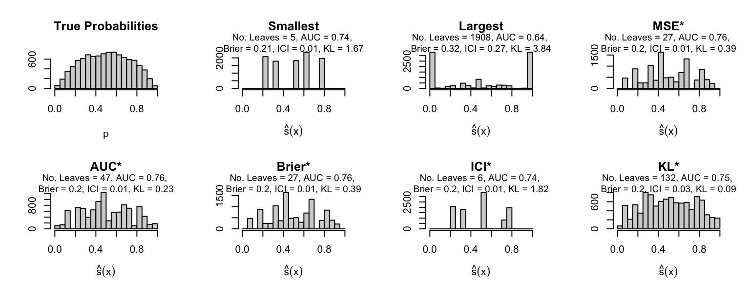
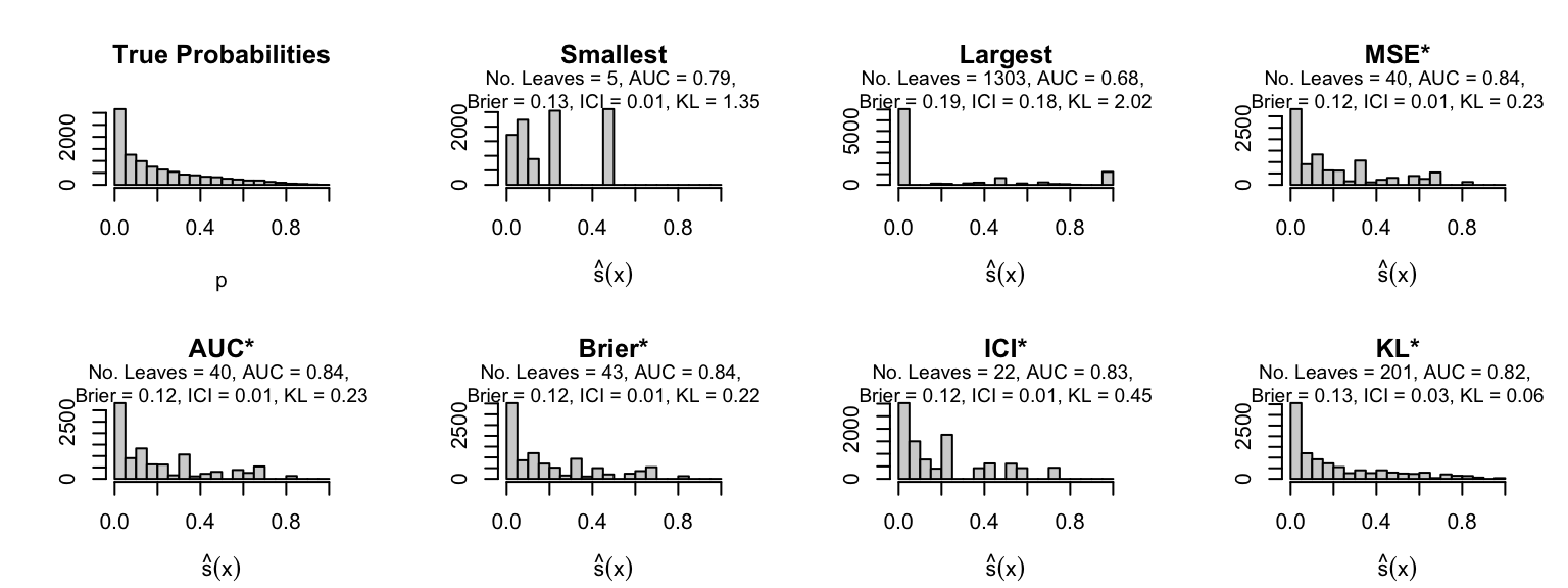
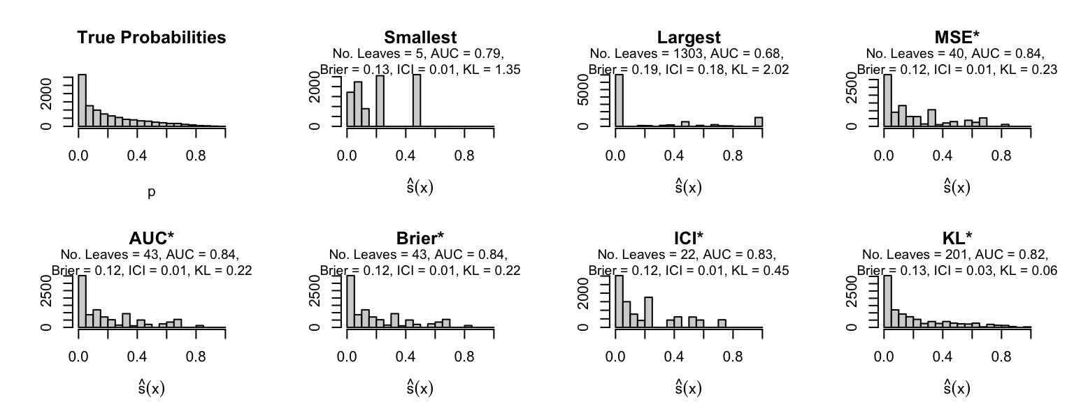
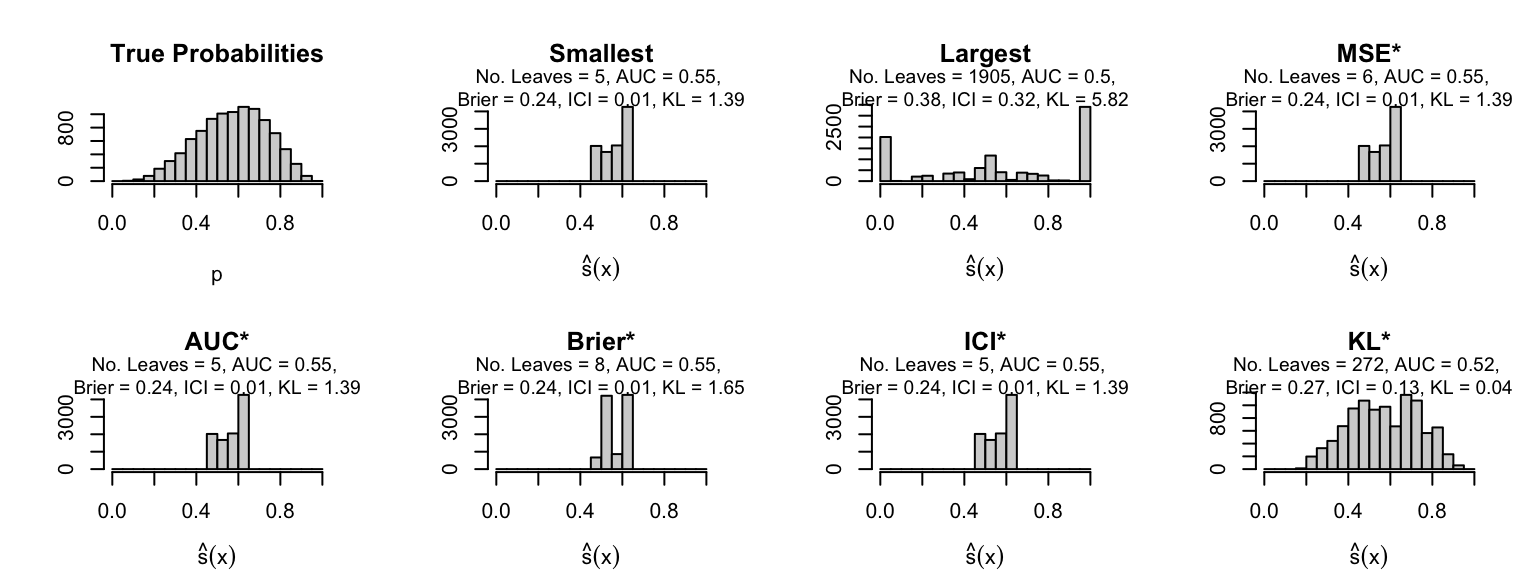
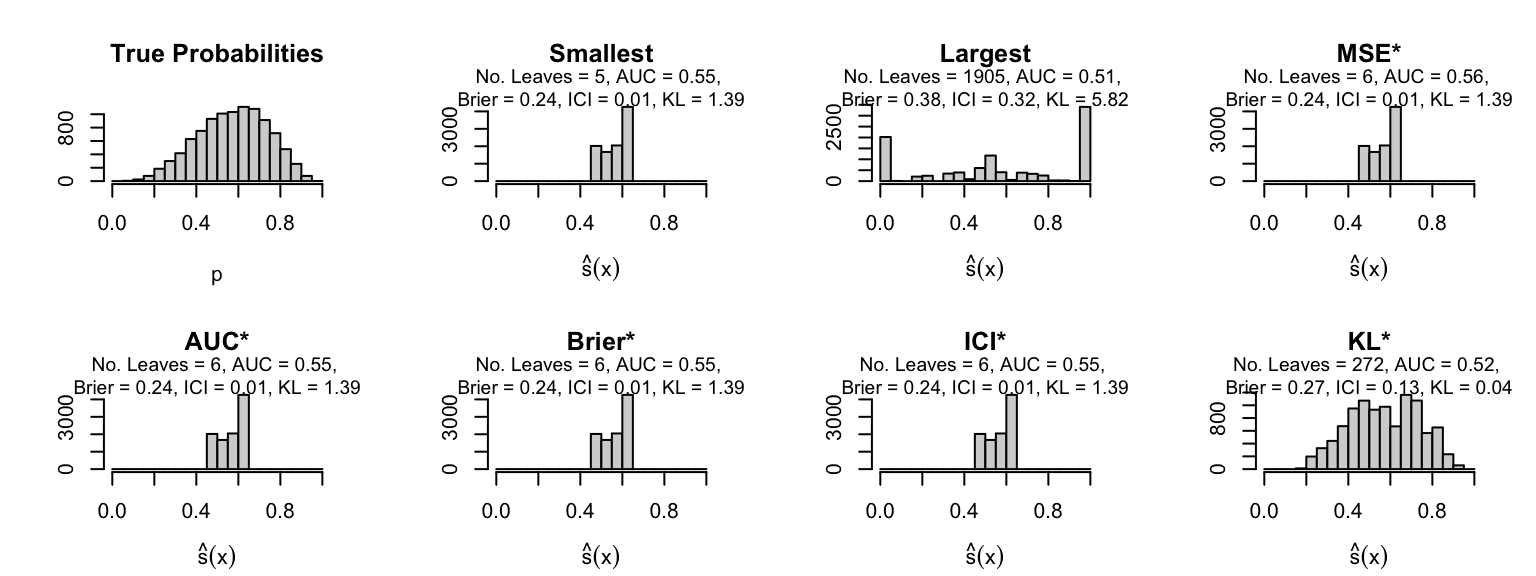
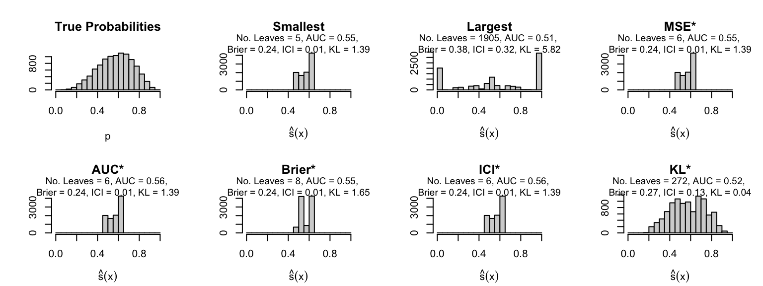
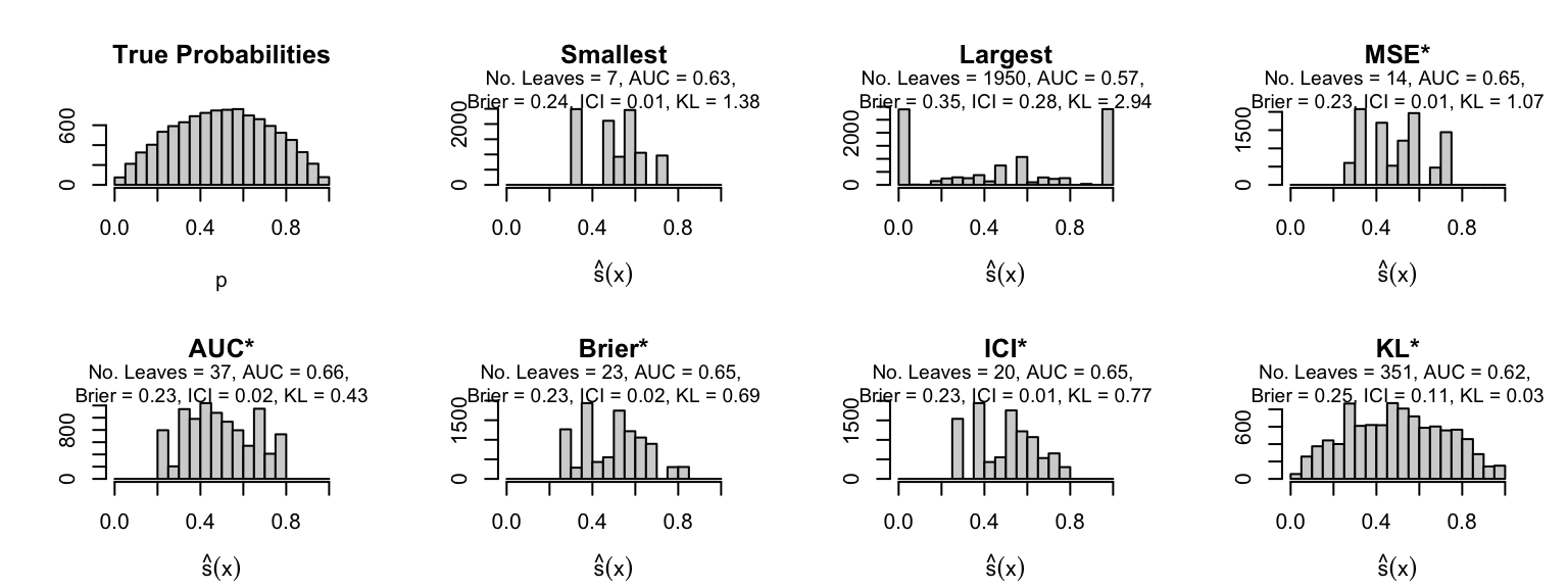
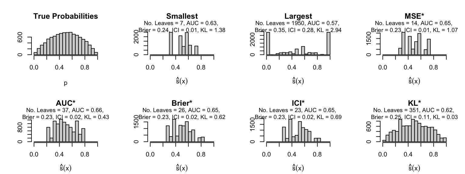
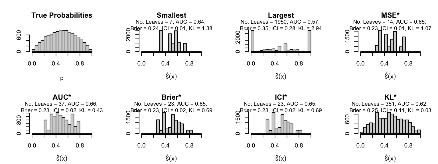
5.5.2.1 Distribution of Scores

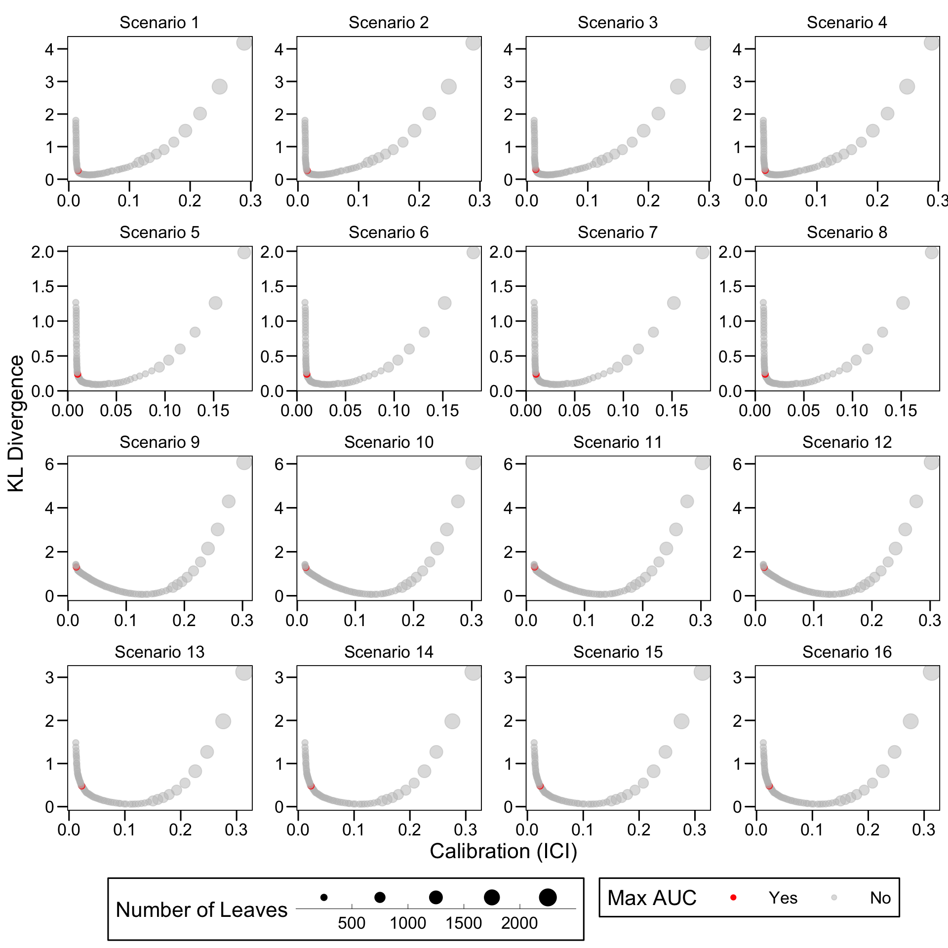
Let us plot the distributions of scores for the trees of interest (smallest, largest, max AUC, min MSE, min KL) for a single replication for each scenario.

Codes to get the barplots

get_bp <- function(interest, 
                   scenario,
                   repn) {
  # Identify the row number of the grid
  tree_of_interest <- 
    trees_of_interest_metrics_tree |> 
    filter(
      result_type == !!interest, 
      scenario == !!scenario,
      repn == !!repn,
      sample == "Test"
    )
  
  ind_grid <- tree_of_interest |> 
    pull("ind")
  
  # The corresponding barplot data
  data_bp <- 
    map(resul_trees[[scenario]], "scores_hist")[[repn]] |> 
    pluck(ind_grid)
  
  subtitle <- str_c(
    "No. Leaves = ", tree_of_interest$nb_leaves, ", ",
    "AUC = ", round(tree_of_interest$AUC, 2), ", \n",
    "Brier = ", round(tree_of_interest$brier, 2), ", ",
    "ICI = ", round(tree_of_interest$ici, 2), ", ",
    "KL = ", round(tree_of_interest$KL_20_true_probas, 2)
  )
  
  plot(
    main = interest,
    data_bp$test, 
    xlab = latex2exp::TeX("$\\hat{s}(x)$"),
    ylab = ""
  )
  mtext(side = 3, line = -0.25, adj = .5, subtitle, cex = .6)
}

plot_hist_scenario <- function(scenario, 
                               repn) {
  par(mfrow = c(2,4), mar = c(4.1, 4.1, 4.1, 2.1))
  # True probabilities
  simu_data <- simulate_data_wrapper(
    scenario = scenario,
    params_df = params_df,
    repn = repn # only one replication here
  )
  true_prob <- simu_data$data$probs_train
  hist(
    true_prob,
    breaks = seq(0, 1, by = .05),
    xlab = "p", ylab = "",
    main = "True Probabilities",
    xlim = c(0, 1)
  )
  
  for (interest in c("Smallest", "Largest", "MSE*" ,"AUC*", "Brier*", "ICI*", "KL*")) {
    get_bp(
      interest = interest, 
      scenario = scenario, 
      repn = repn
    )
  }
}

We only show the distributions for the first replication.

repn <- 1

Code

save_graph <- FALSE
if (save_graph) {
  cairo_pdf("figures/tree-scenario1-hist-scores.pdf", width  = 8, height = 3)
}
plot_hist_scenario(scenario = 1, repn = repn)

Distribution of true probabilities and estimated scores on test set for trees of interest (0 noise variables).

Code

if (save_graph) dev.off()

Code

plot_hist_scenario(scenario = 2, repn = repn)

Distribution of true probabilities and estimated scores on test set for trees of interest (10 noise variables).

Code

plot_hist_scenario(scenario = 3, repn = repn)

Distribution of true probabilities and estimated scores on test set for trees of interest (50 noise variables).

Code

plot_hist_scenario(scenario = 4, repn = repn)

Distribution of true probabilities and estimated scores on test set for trees of interest (100 noise variables).

Code

plot_hist_scenario(scenario = 5, repn = repn)

Code

plot_hist_scenario(scenario = 6, repn = repn)

Code

plot_hist_scenario(scenario = 7, repn = repn)

Code

plot_hist_scenario(scenario = 8, repn = repn)

Distribution of true probabilities and estimated scores on test for trees of interest (100 noise variables).

Code

plot_hist_scenario(scenario = 9, repn = repn)

Code

plot_hist_scenario(scenario = 10, repn = repn)

Code

plot_hist_scenario(scenario = 11, repn = repn)

Code

plot_hist_scenario(scenario = 12, repn = repn)

Code

plot_hist_scenario(scenario = 13, repn = repn)

Code

plot_hist_scenario(scenario = 14, repn = repn)

Code

plot_hist_scenario(scenario = 15, repn = repn)

Code

plot_hist_scenario(scenario = 16, repn = repn)

5.5.2.2 Metrics vs Number of Leaves

We can plot some metrics (AUC, ICI, KL) as a function of the average number of leaves in the trees.

Codes to get the plots

plot_metric_leaves <- function(dgp) {
  data_plot <-
    metrics_trees_all |>
    mutate(
      dgp = case_when(
        scenario %in% 1:4 ~ 1,
        scenario %in% 5:8 ~ 2,
        scenario %in% 9:12 ~ 3,
        scenario %in% 13:16 ~ 4
      ),
      no_noise = c(0, 10, 50, 100)[(scenario-1)%%4 + 1],
      no_noise = factor(
        no_noise, levels = c(no_noise),
        labels = str_c(no_noise, " noise variables")
      )
    ) |>
    filter(dgp == !!dgp) |>
    group_by(
      sample, dgp, no_noise, scenario, ind, min_bucket
    ) |>
    summarise(
      KL_20_true_probas = mean(KL_20_true_probas),
      auc = mean(AUC),
      brier = mean(brier),
      ici = mean(ici),
      nb_leaves = mean(nb_leaves),
      .groups = "drop"
    ) |>
    pivot_longer(cols = c(auc, brier, ici, KL_20_true_probas), names_to = "metric") |>
    mutate(metric = factor(
      metric,
      levels = c("auc", "brier" ,"ici", "KL_20_true_probas"),
      labels = c("AUC", "Brier", "ICI", "KL Divergence")
    ))

  ggplot(
    data = data_plot |> arrange(nb_leaves),
    mapping = aes(x = nb_leaves, y = value)
  ) +
    geom_line(
      mapping = aes(colour = sample, group = )
    ) +
    ggh4x::facet_grid2(metric~no_noise, scales = "free_y", independent = "y") +
    scale_colour_manual(
      "Sample", values = colour_samples,
      labels = c("Train", "Validation", "Test")
    ) +
    theme_paper() +
    labs(x = "Average Number of leaves", y = NULL)
}

Code

plot_metric_leaves(dgp = 1)

Metrics depending on the average number of leaves in the estimated trees (DGP 1)

Code

plot_metric_leaves(dgp = 2)

Metrics depending on the average number of leaves in the estimated trees (DGP 2)

Code

plot_metric_leaves(dgp = 3)

Metrics depending on the average number of leaves in the estimated trees (DGP 3)

Code

plot_metric_leaves(dgp = 4)

Metrics depending on the average number of leaves in the estimated trees (DGP 4)

5.5.2.3 Relationship between calibration, KL divergence and tree complexity

For a given scenario, each dot in the figures below is obtained by computing the average metrics on the 100 replications.

Codes to get the plots

data_plot <- metrics_trees_all |> 
  group_by(
    sample, scenario, ind
  ) |> 
  summarise(
    KL_20_true_probas = mean(KL_20_true_probas),
    ici = mean(ici),
    nb_leaves = mean(nb_leaves),
    AUC = mean(AUC)
  ) |> 
  filter(sample=="Test") |> 
  mutate(
    scenario_lab = factor(str_c("Scenario ", scenario)),
    scenario_lab = fct_reorder(scenario_lab, scenario)
  ) |> 
  group_by(
    sample, scenario
  ) |> 
  mutate(
    is_max_auc = AUC == max(AUC),
    is_max_auc = factor(is_max_auc, levels = c(TRUE, FALSE), labels = c("Yes", "No"))
  ) |> 
  ungroup()

ggplot(
  data = data_plot,
  mapping = aes(
    x = ici, y = KL_20_true_probas, group = sample
  )
) + 
  geom_point(
    mapping = aes(
      size = nb_leaves,
      colour = is_max_auc, fill = is_max_auc, alpha = is_max_auc)
    ) +
  facet_wrap(~scenario_lab, ncol = 4, scales = "free") +
  labs(x = "Calibration (ICI)", y = "KL Divergence") +
  scale_size_binned_area("Number of Leaves") +
  scale_colour_manual(
    "Max AUC", values = c("Yes" = "red", "No" = "gray")
  ) +
  scale_fill_manual(
    "Max AUC", values = c("Yes" = "red", "No" = "gray")
  ) +
  scale_alpha_manual(
    "Max AUC", values = c("Yes" = 1, "No" = .5)
  ) +
  theme_paper() +
  theme(legend.key.width = unit(1.5, "cm"))

Figure 5.1: Kullback-Leibler divergence between estimated scores and true probabilities vs. calibration, for various tree depths (Test set).

Let us also visualize this using ggplot2 instead.

Codes to get the plots

plot_kl_vs_calib <- function(scenario_number, 
                             calib_metric,
                             log_scale = FALSE) {
  data_plot <- metrics_trees_all |> 
    filter(scenario == !!scenario_number) |> 
    group_by(sample, scenario, ind) |> 
    summarise(
      KL_20_true_probas = mean(KL_20_true_probas),
      ici = mean(ici),
      brier = mean(brier),
      nb_leaves = mean(nb_leaves),
      auc = mean(AUC),
      .groups = "drop"
    )
  
  data_plot_max_auc <- 
    data_plot |> 
    filter(sample == "Test") |> 
    group_by(sample, scenario) |>
    mutate(is_max_auc = auc == max(auc)) |> 
    ungroup() |> 
    filter(is_max_auc == TRUE) |> 
    select(sample, scenario, !!calib_metric, KL_20_true_probas)
  
  x_lab <- latex2exp::TeX(
    str_c(
    "Calibration (", ifelse(calib_metric == "ici", "ICI", "Brier Score"),
    ifelse(log_scale == TRUE, ", log scale)", ")")
    )
  )
  
  p <- ggplot(
    data = data_plot |> arrange(nb_leaves),
    mapping = aes(
      x = !!sym(calib_metric), y = KL_20_true_probas
    )
  ) + 
    geom_path(
      mapping = aes(colour = sample),
      arrow = arrow(type = "closed", ends = "last", 
                    length = unit(0.08, "inches"))
    ) +
    geom_vline(
      data = data_plot_max_auc,
      mapping = aes(xintercept = !!sym(calib_metric)),
      linetype = "dashed"
    ) +
    geom_hline(
      data = data_plot_max_auc,
      mapping = aes(yintercept = KL_20_true_probas),
      linetype = "dashed"
    ) +
    scale_colour_manual("Sample", values = colour_samples, 
                        labels = c("Train", "Validation", "Test")) +
    labs(x = x_lab, y = "KL Divergence") +
    scale_size_binned_area("Number of Leaves") +
    theme_paper() +
    theme(legend.key.width = unit(1.5, "cm"))
  
  if (log_scale) p <- p + scale_x_log10() + scale_y_log10()
  p
}

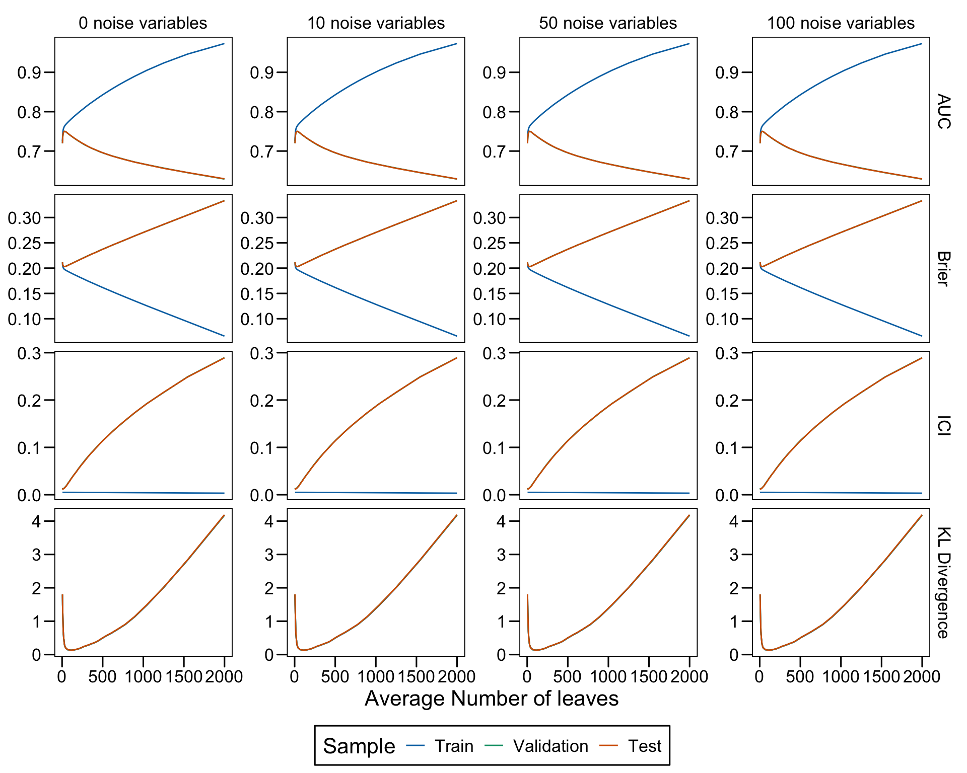
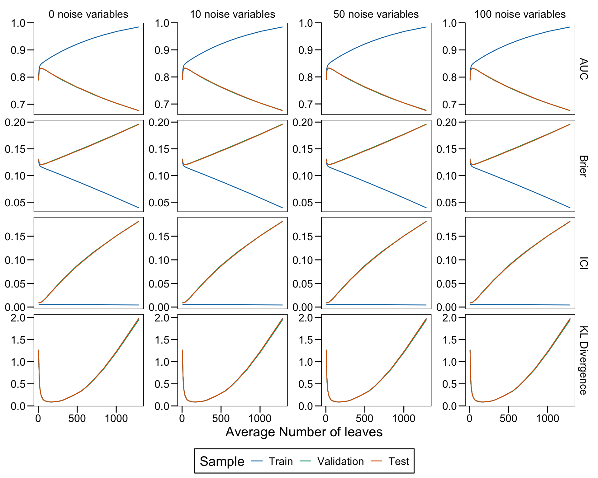
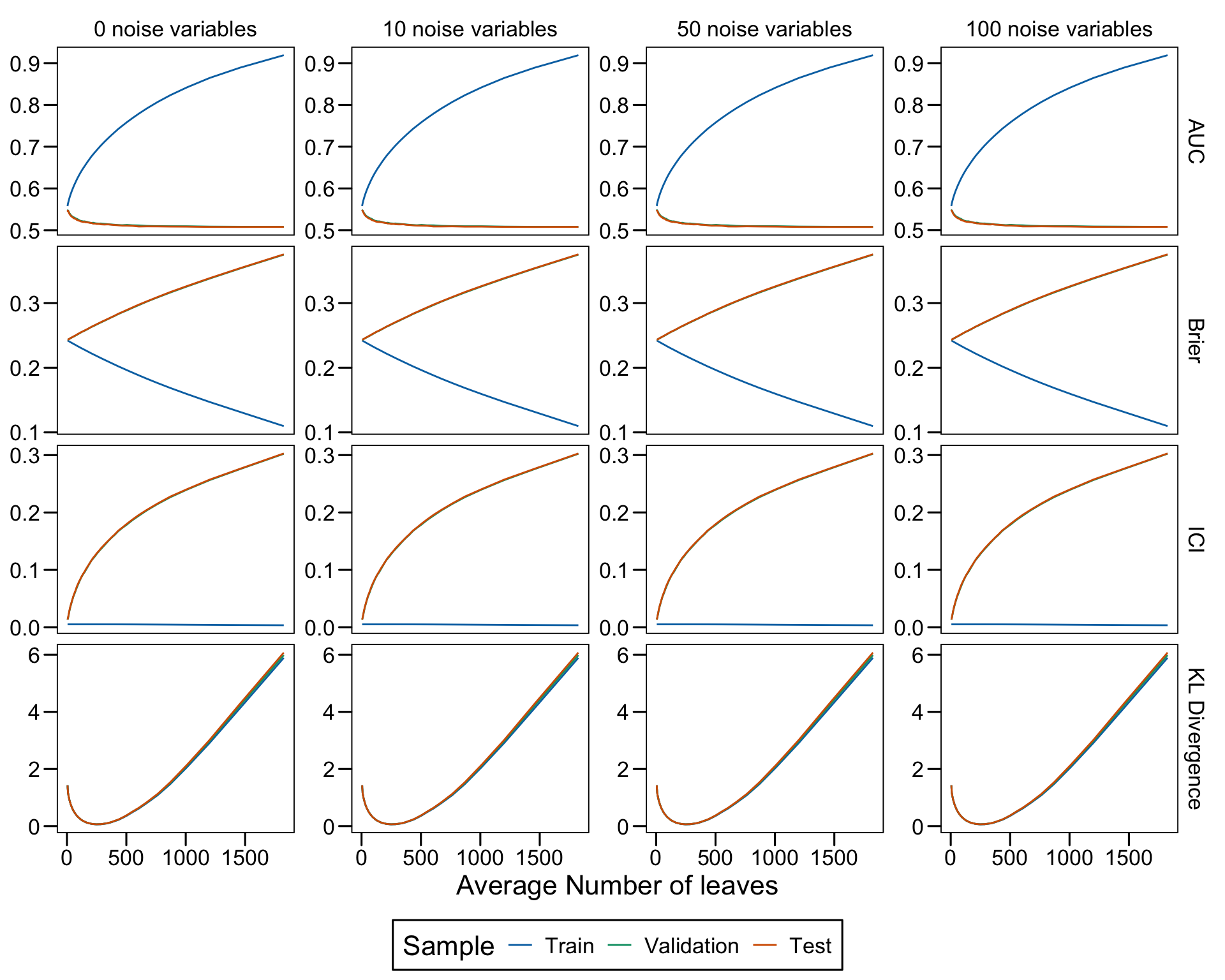
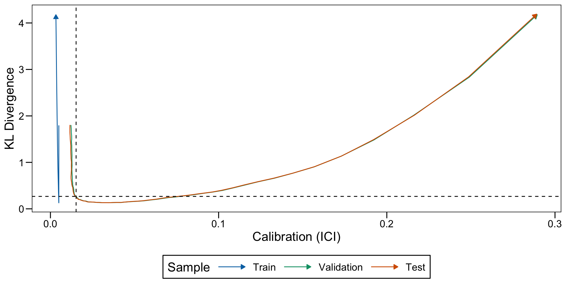
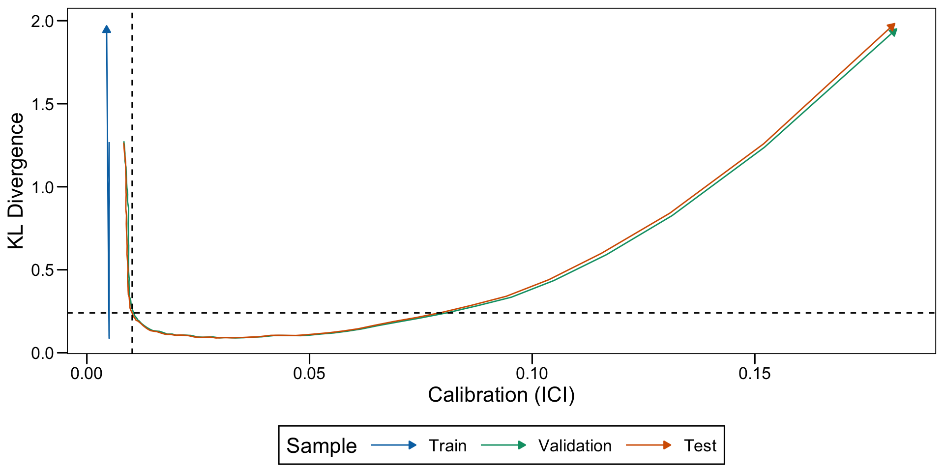
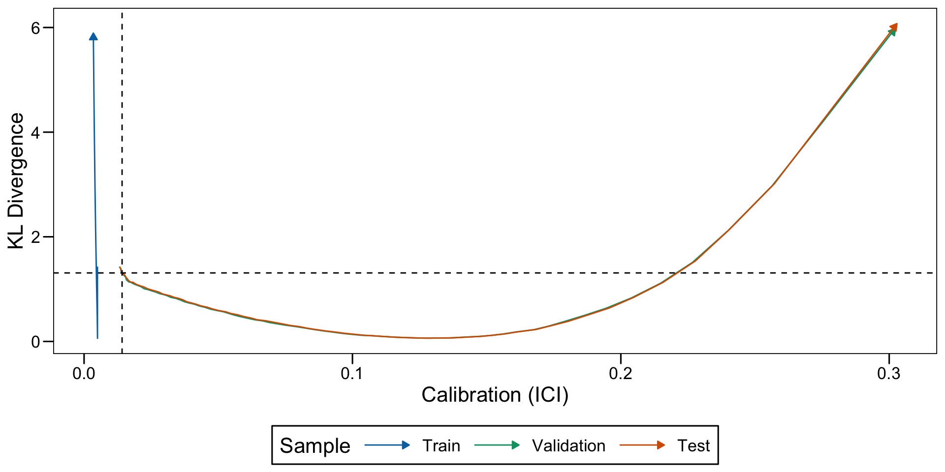
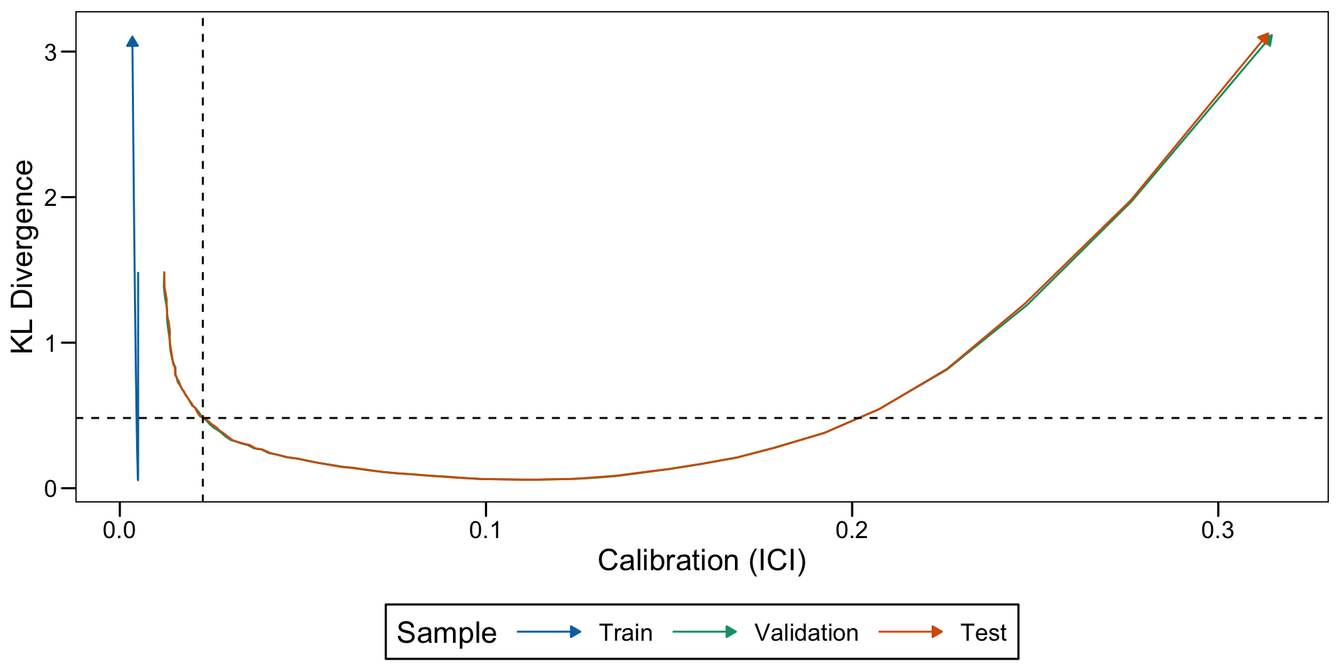
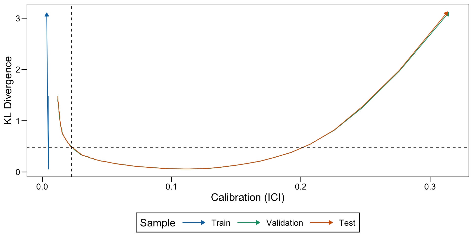
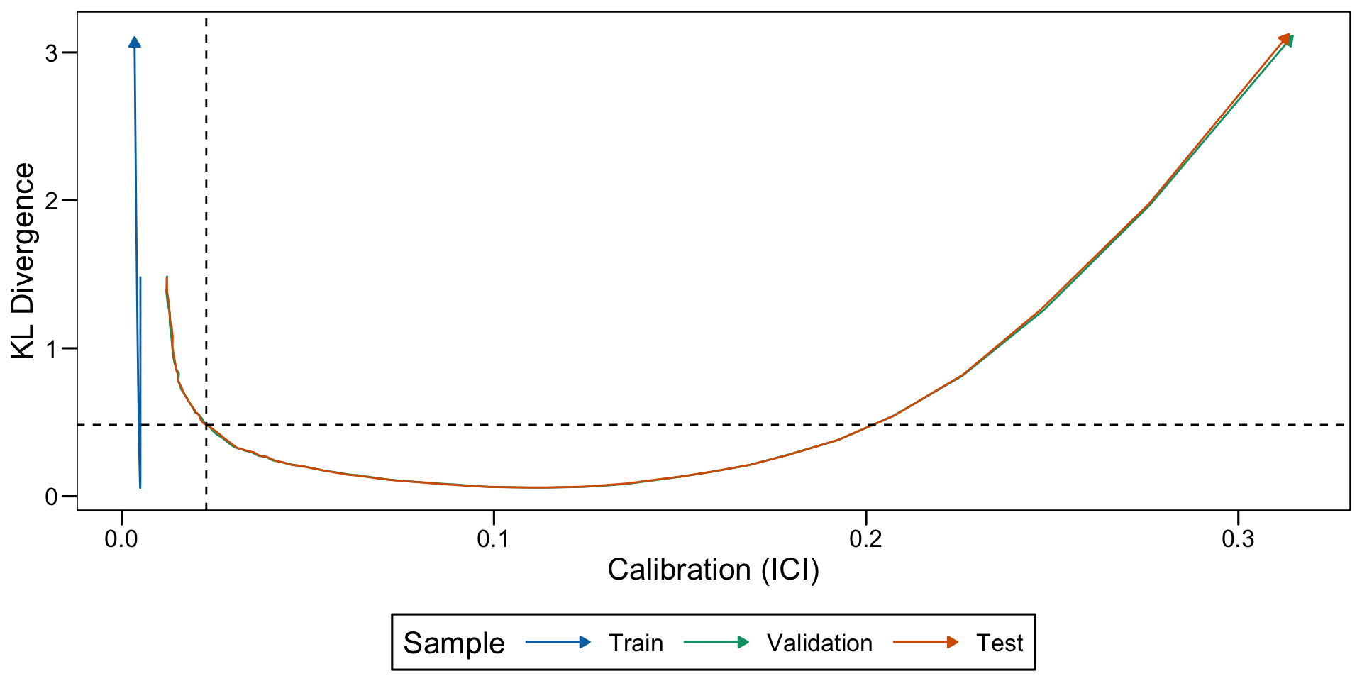
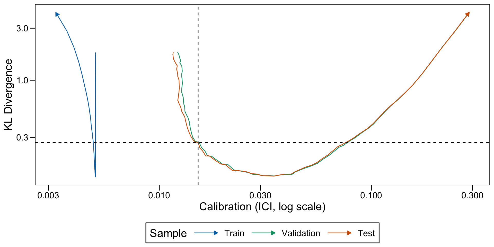
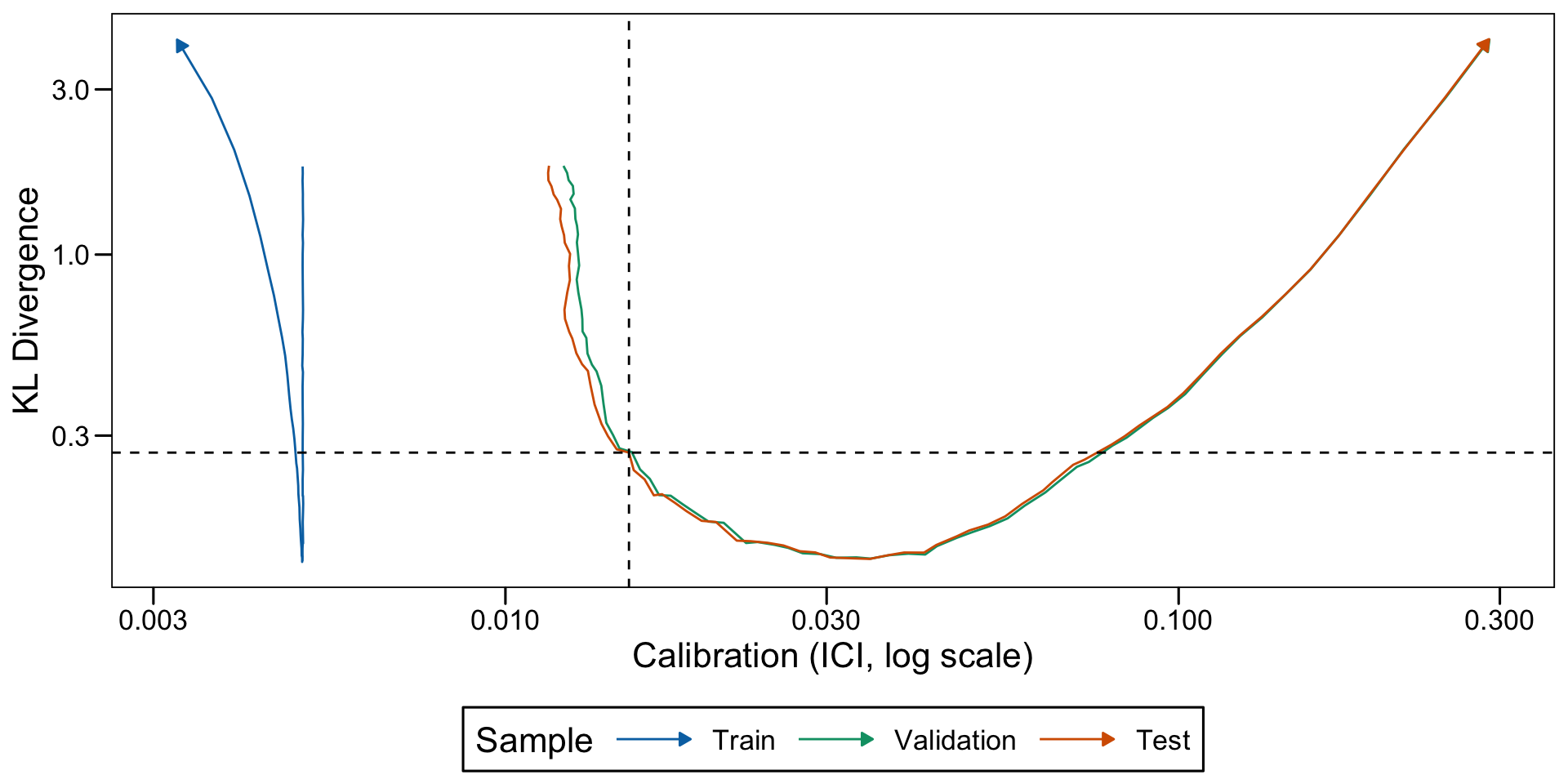
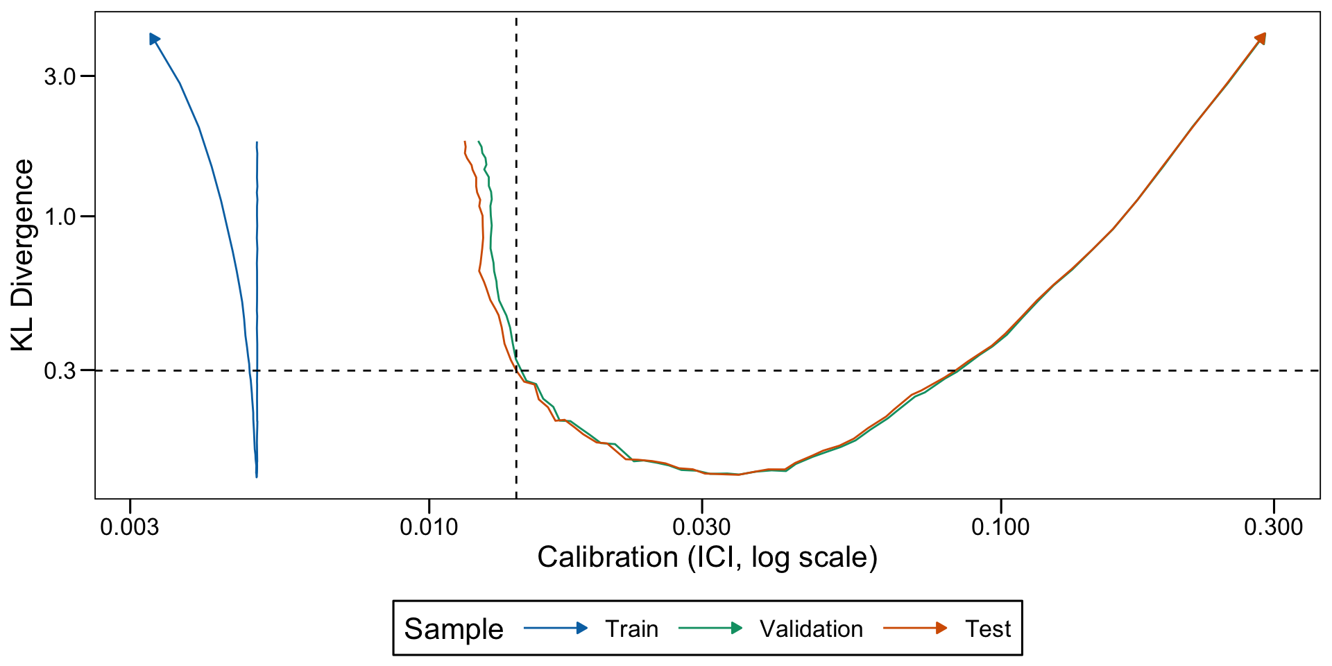
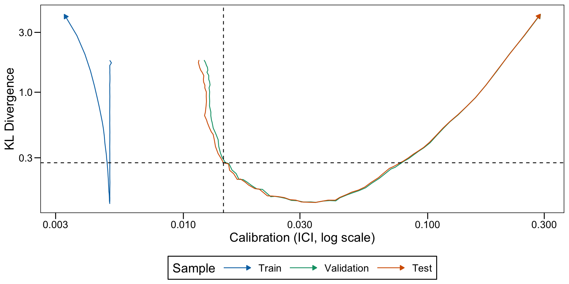
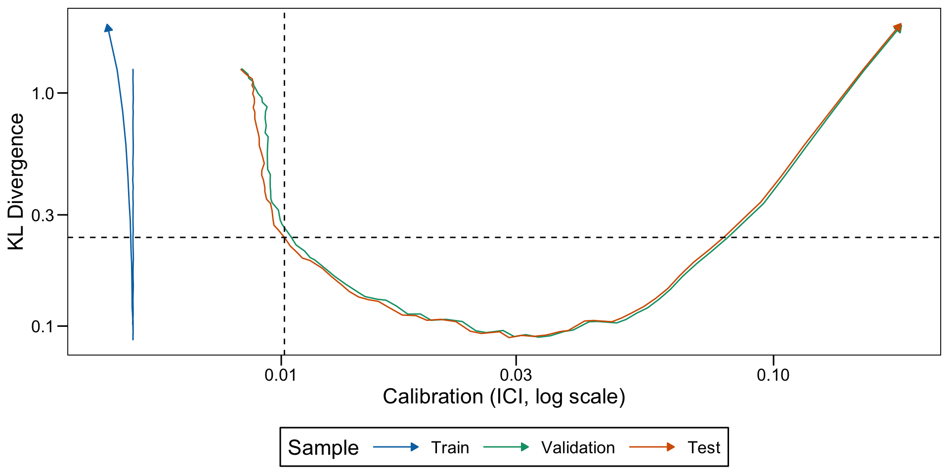
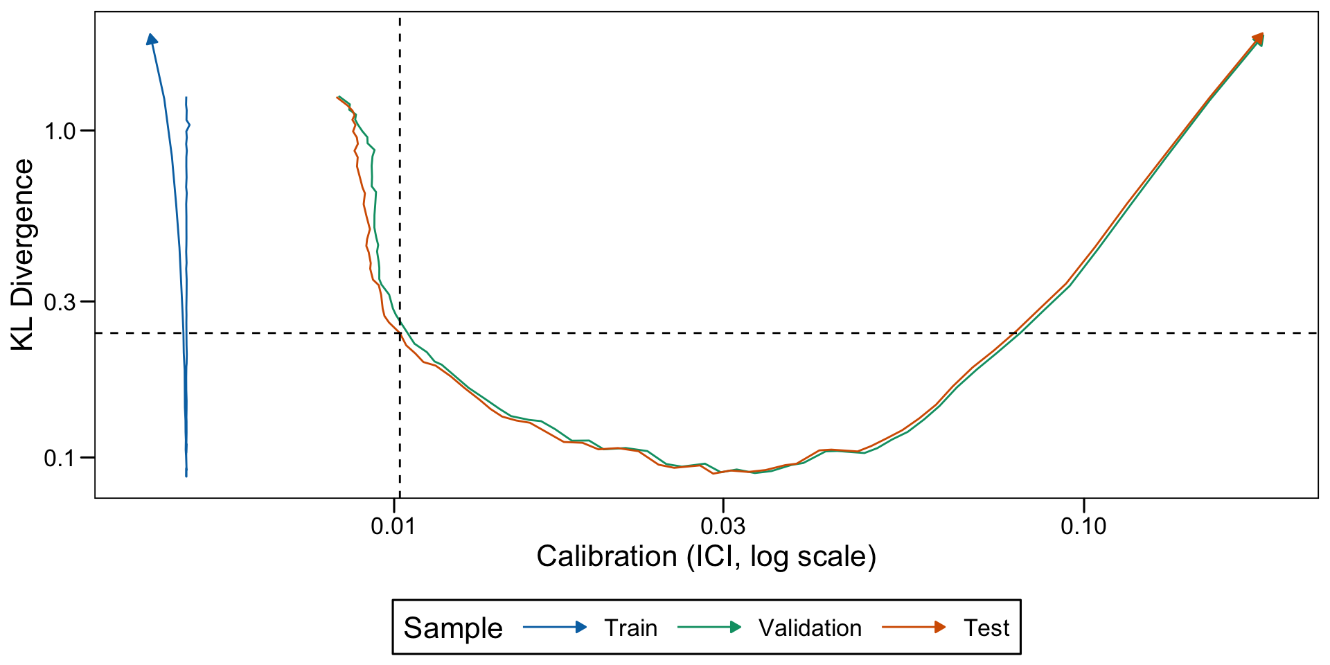
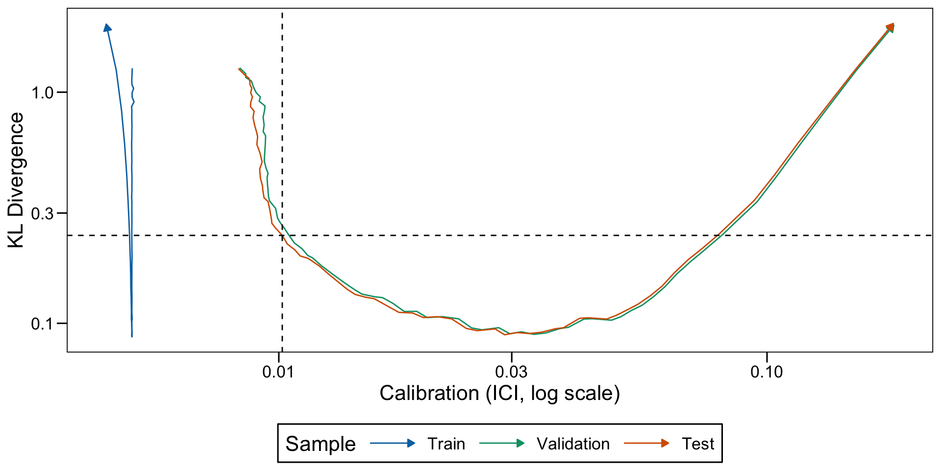
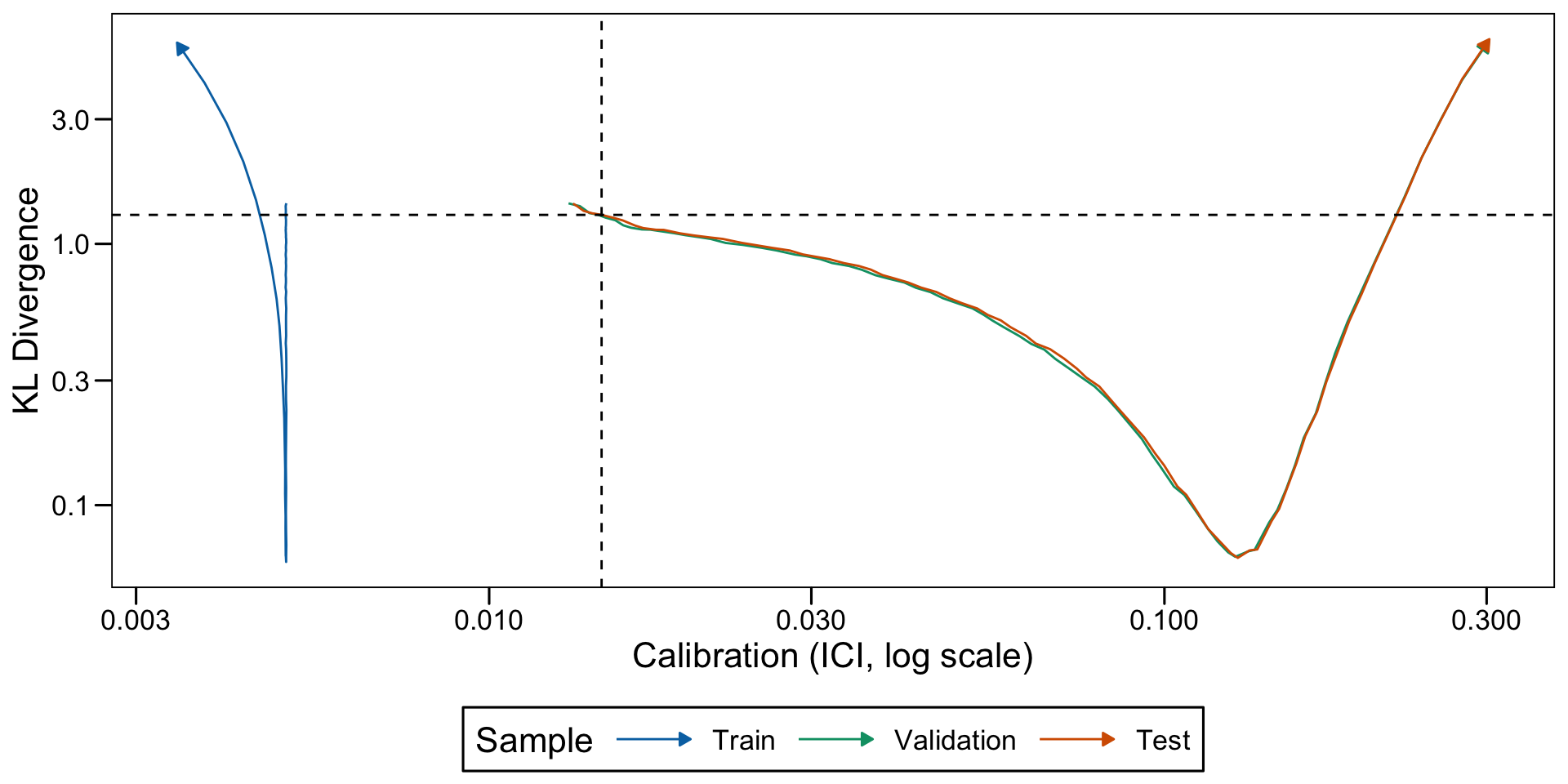
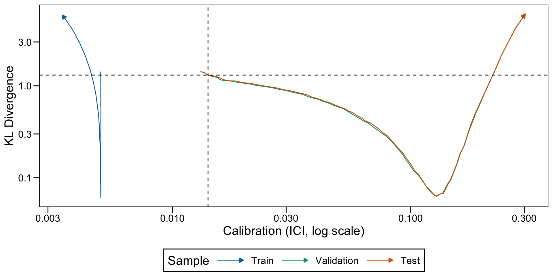
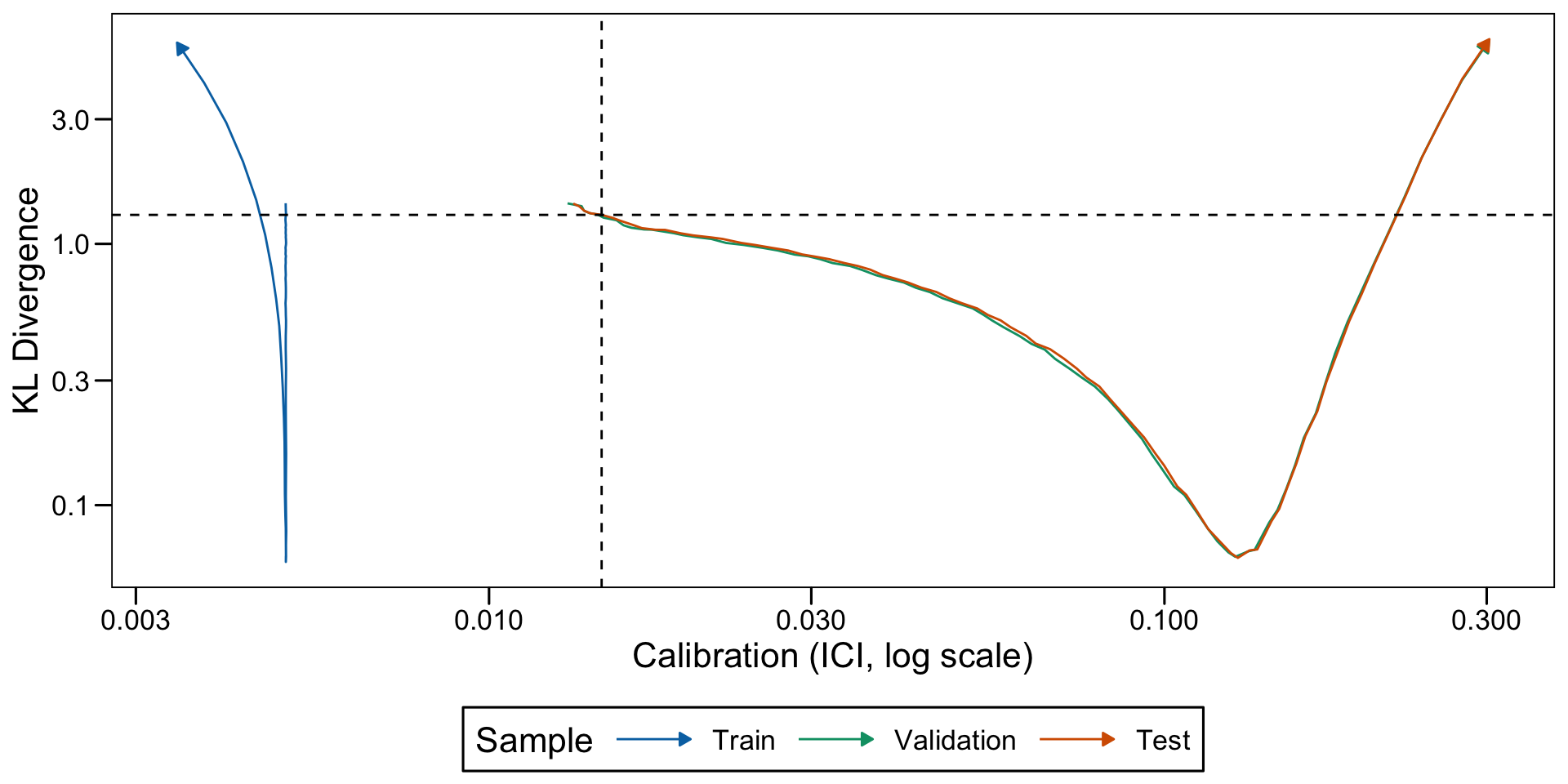
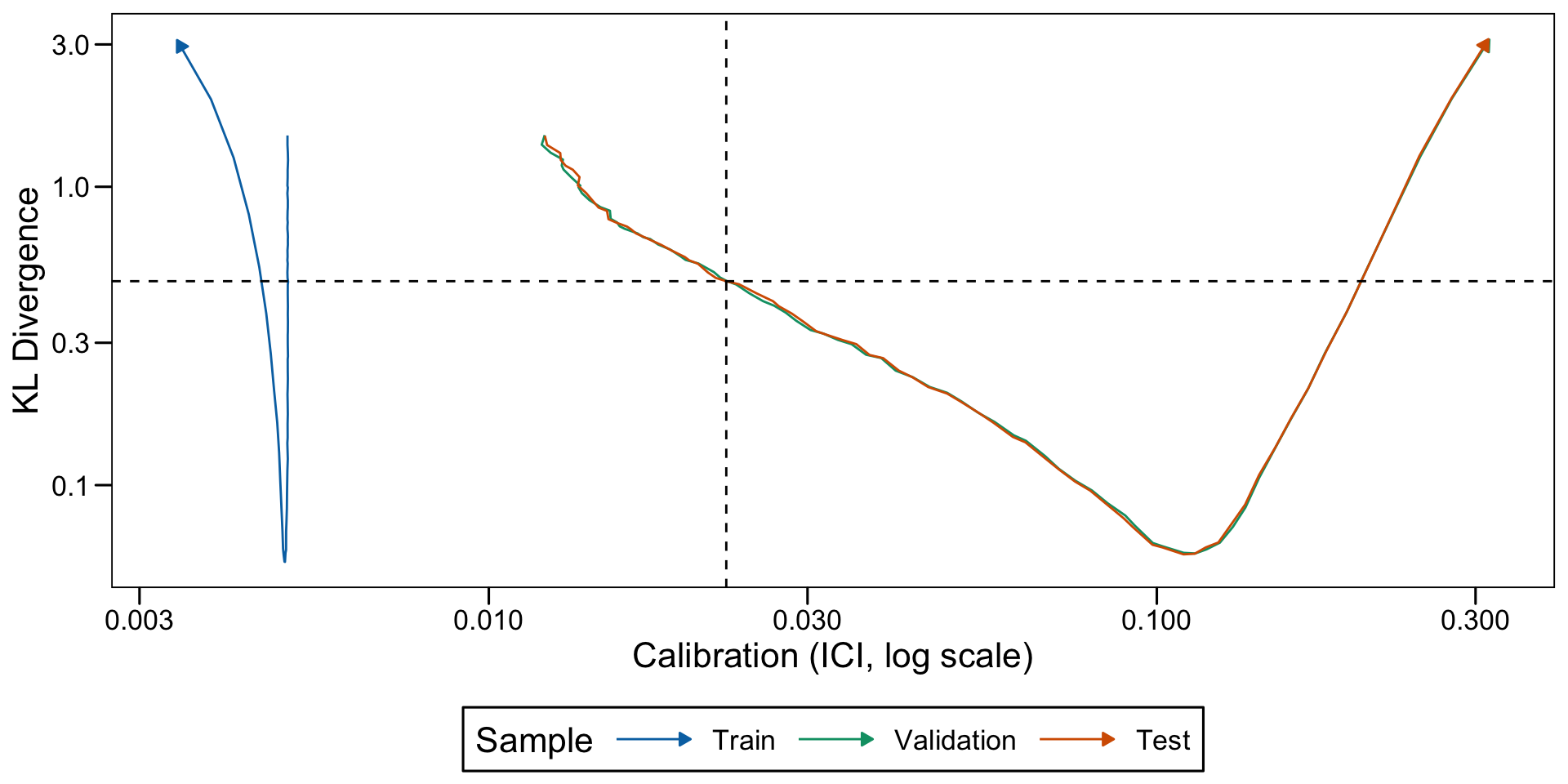
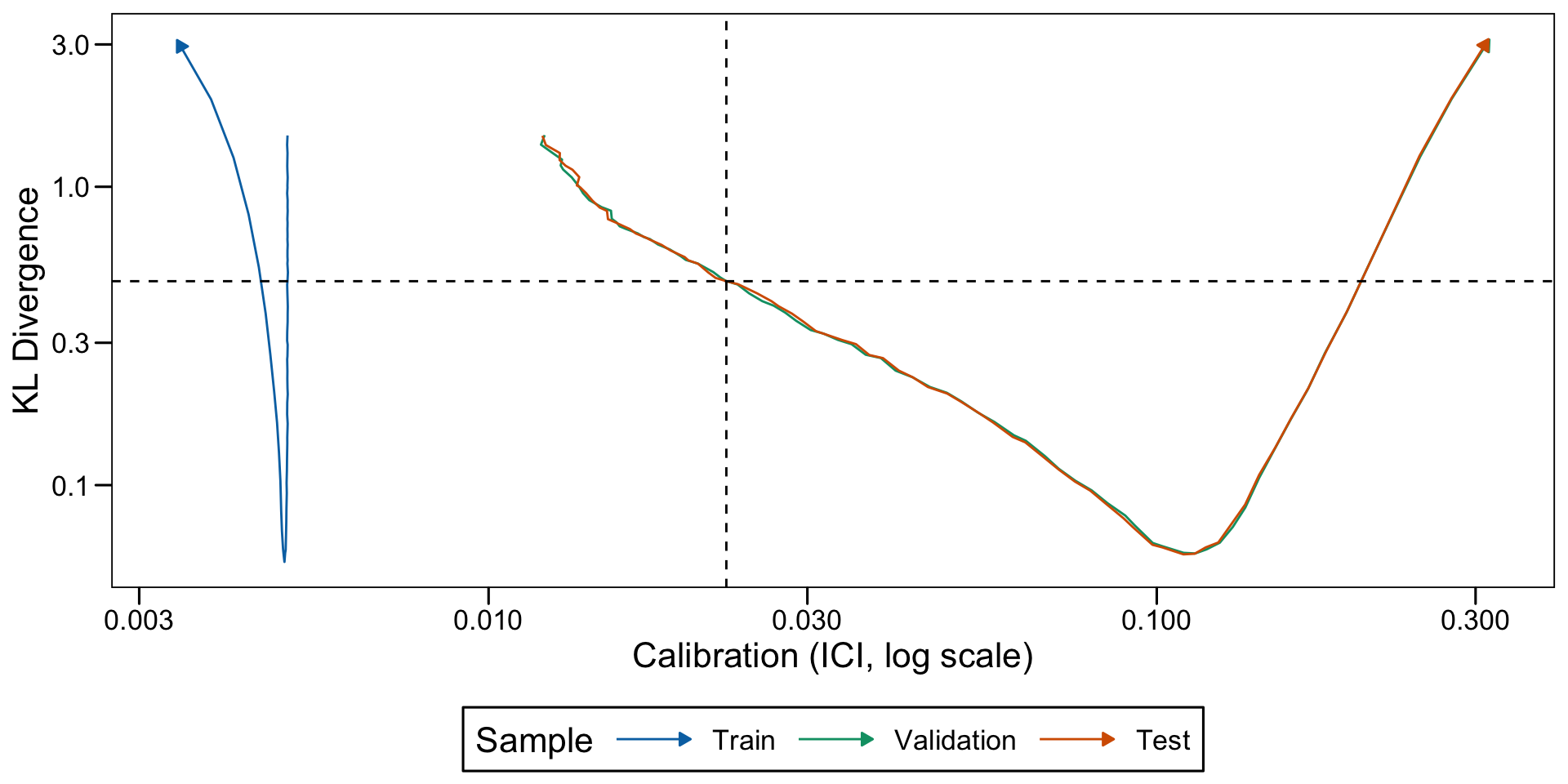
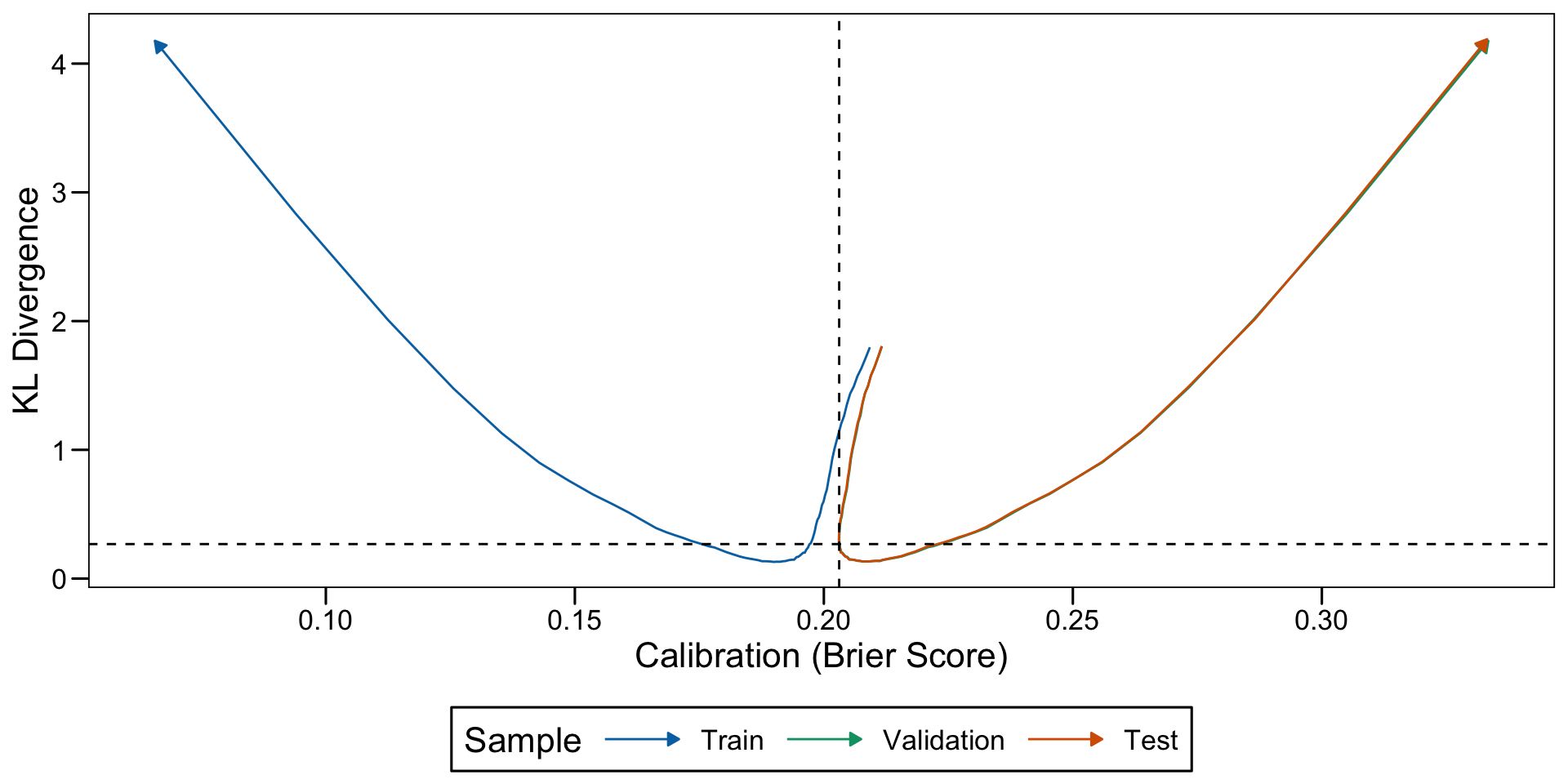
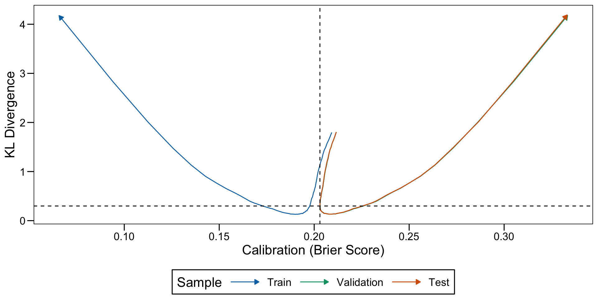
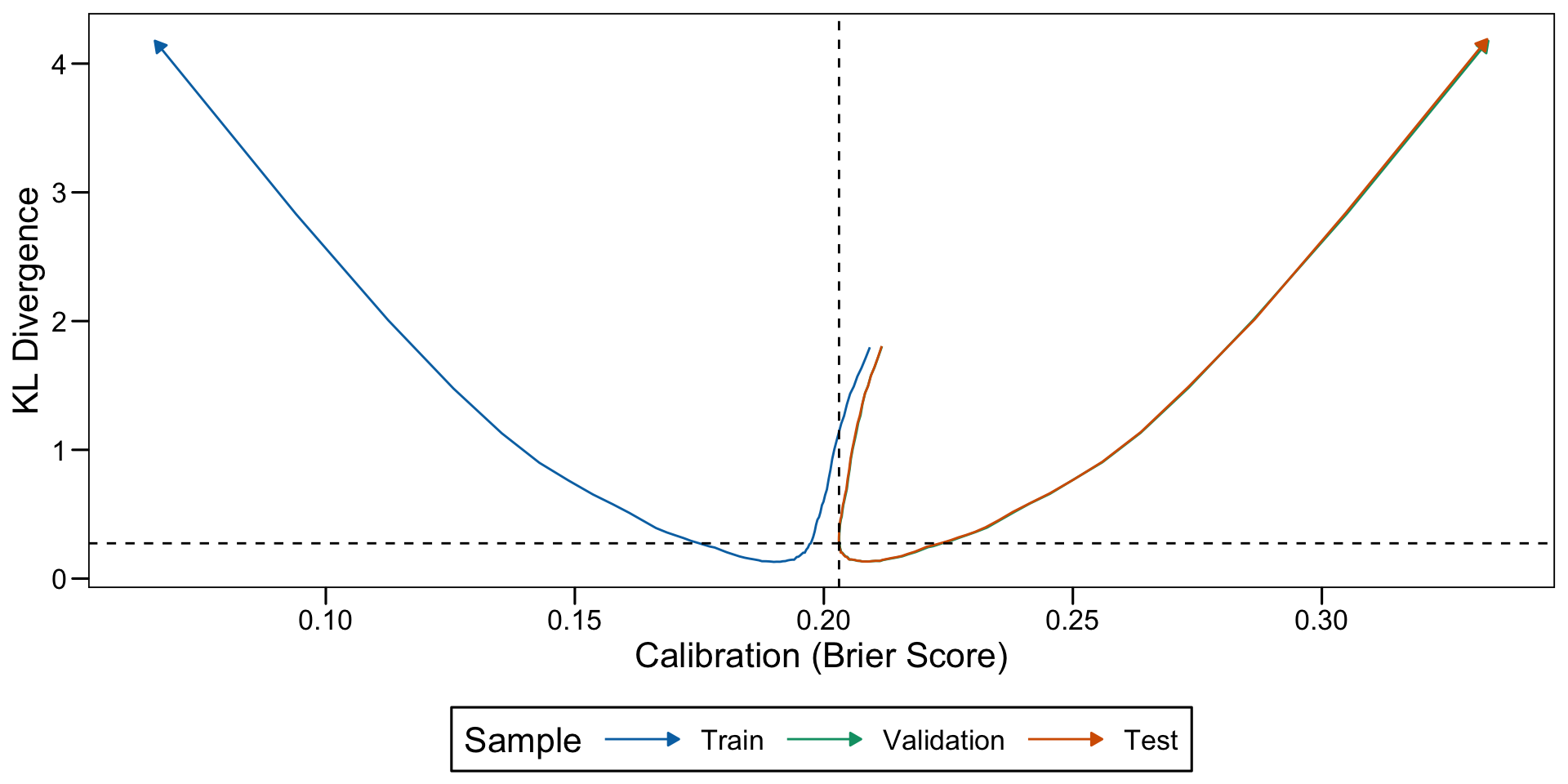
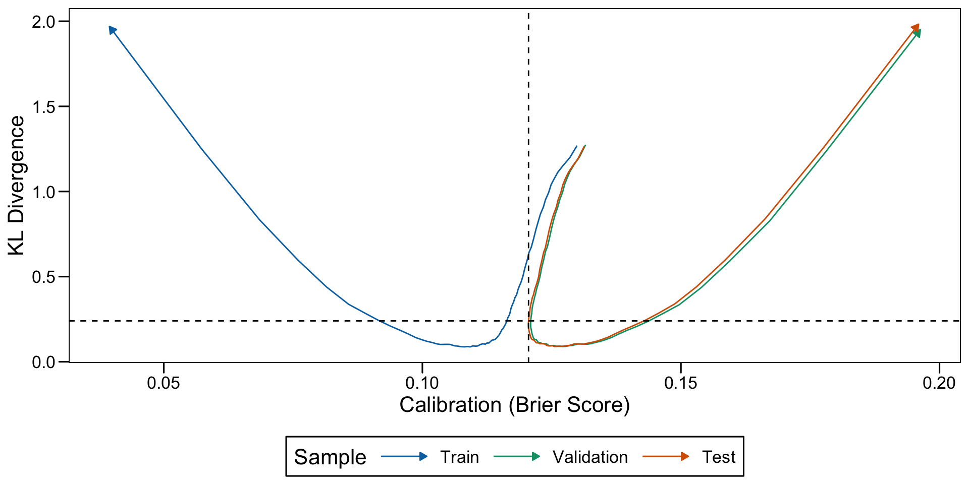
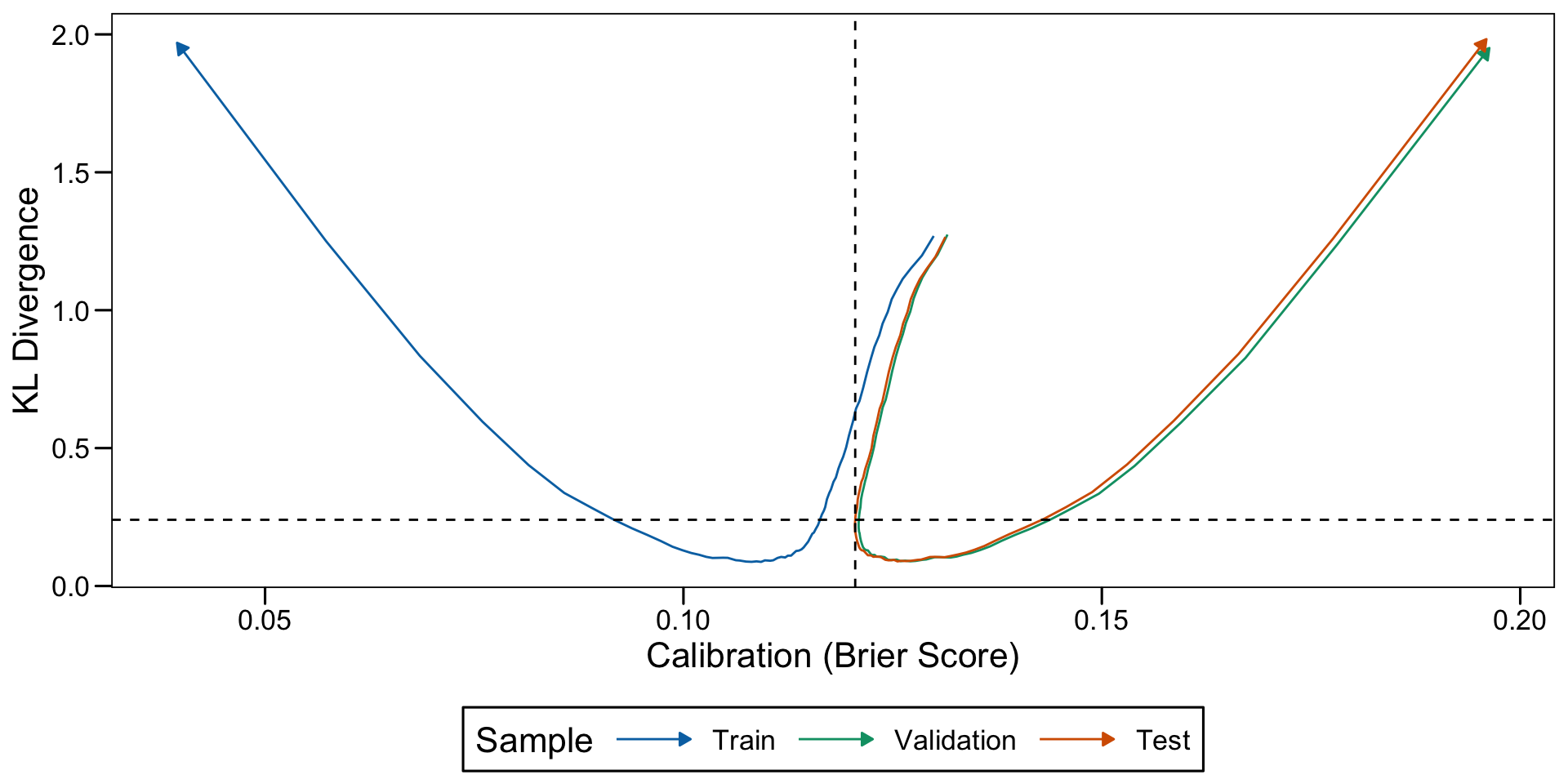
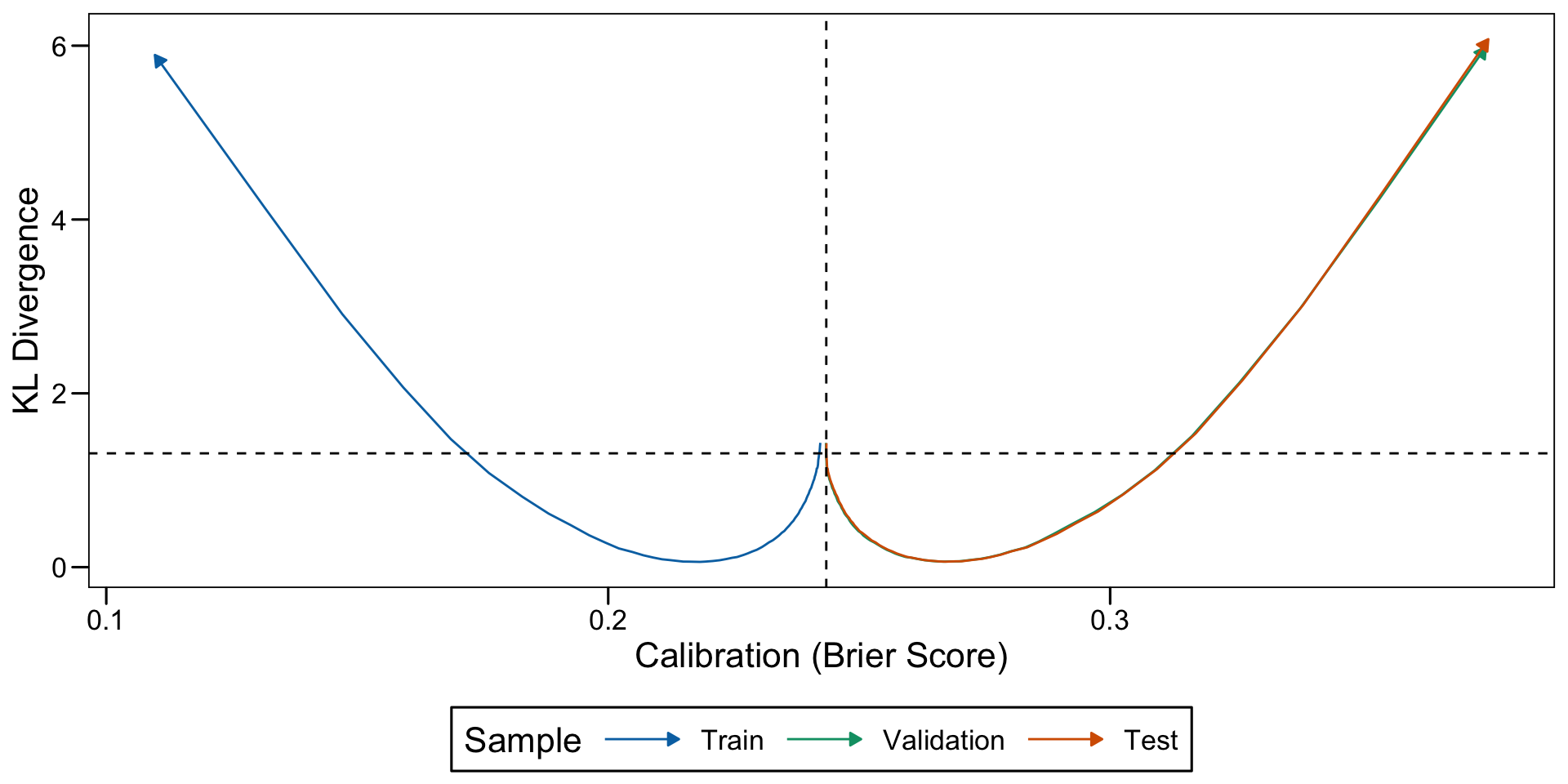
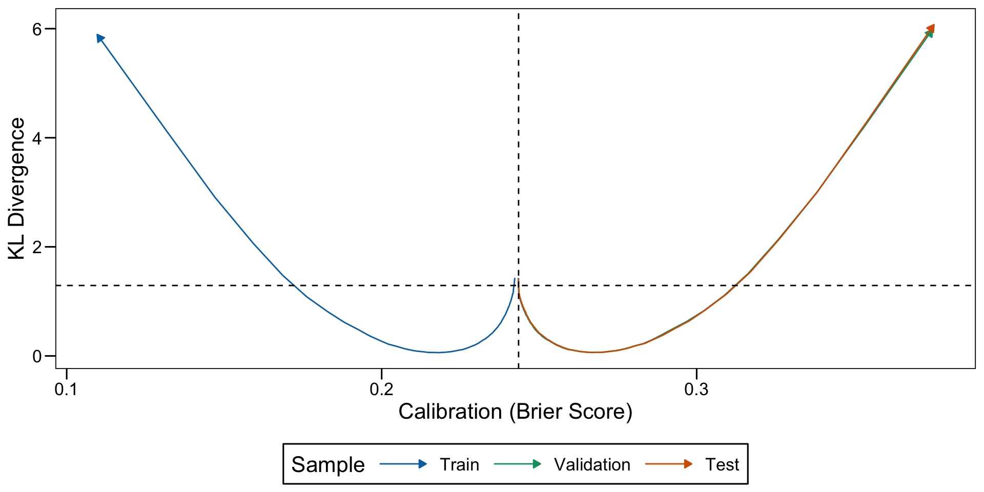
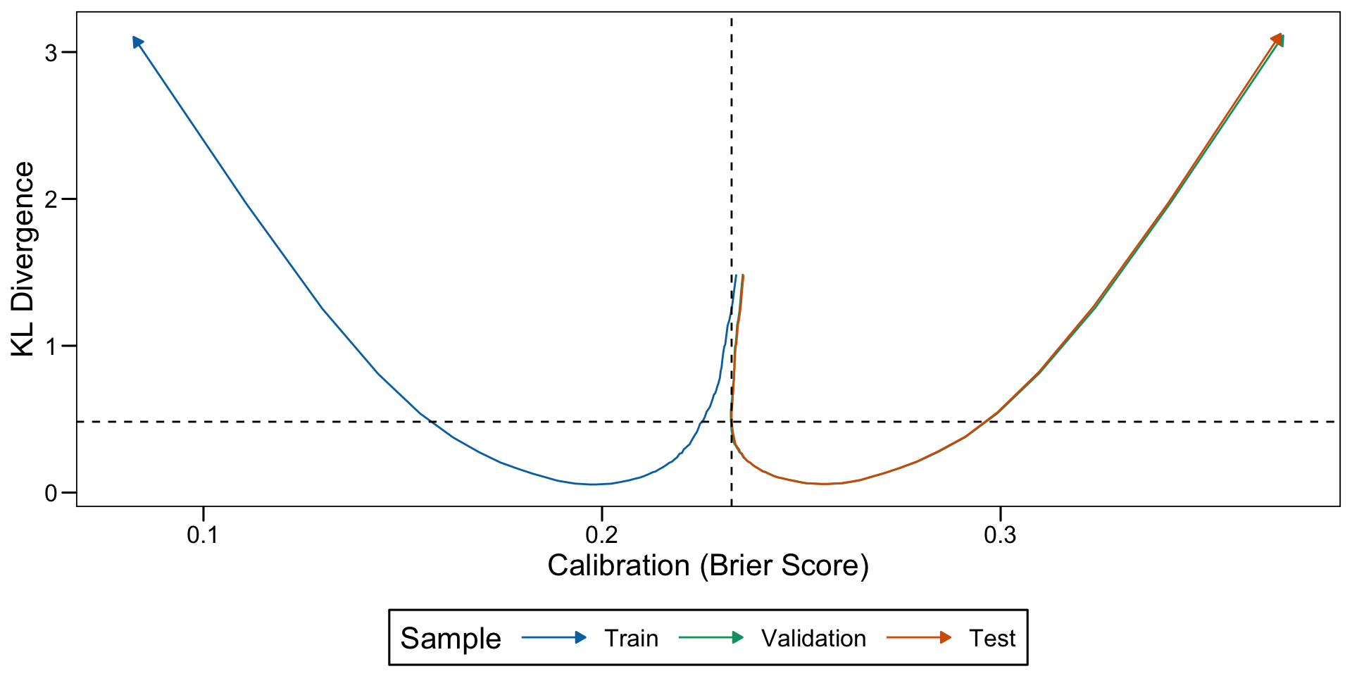
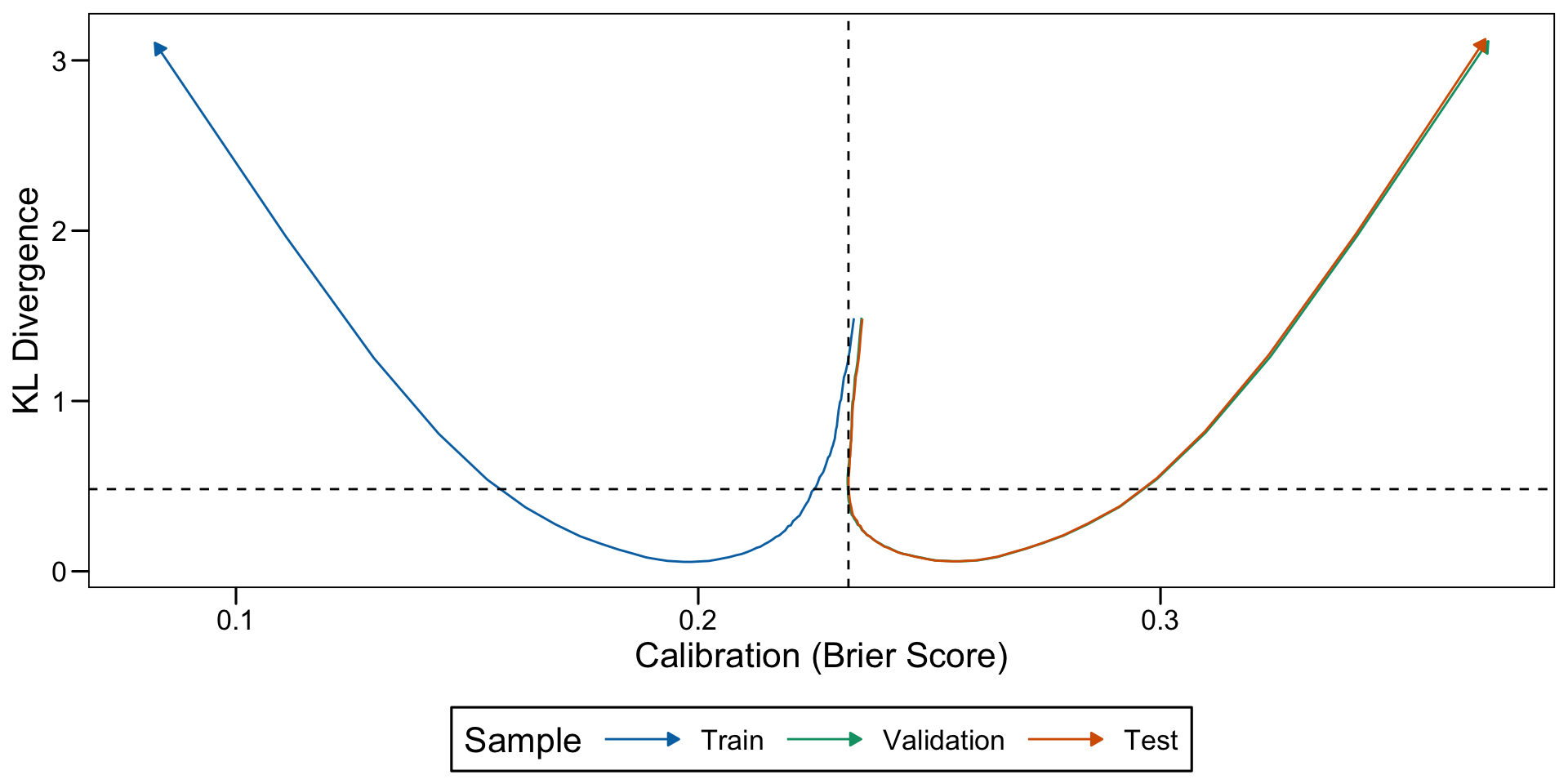
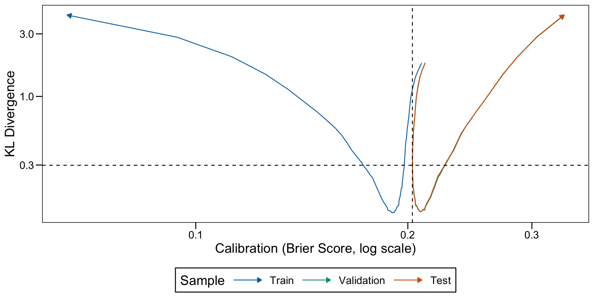
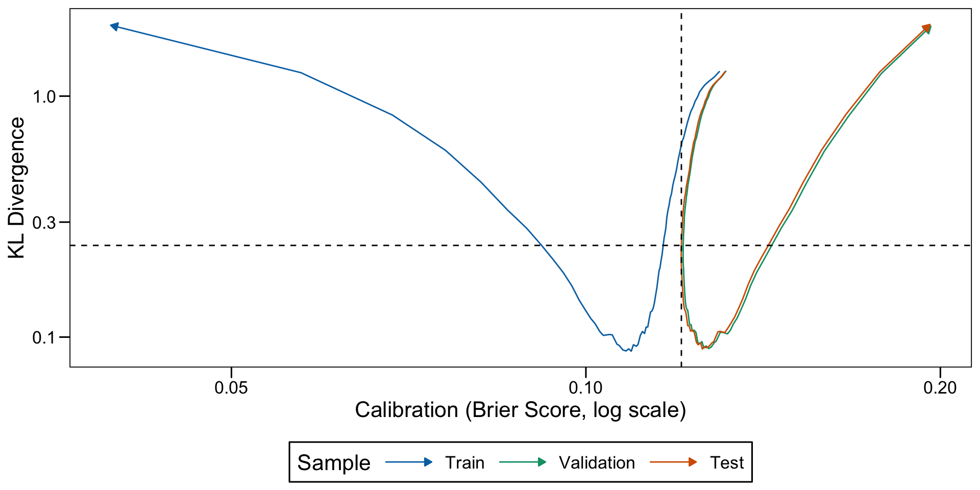
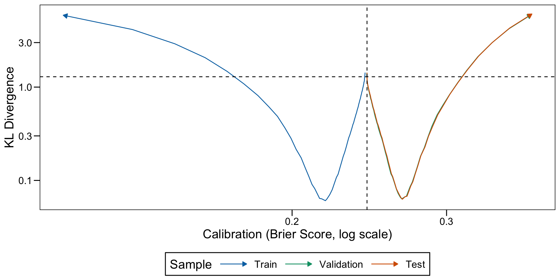
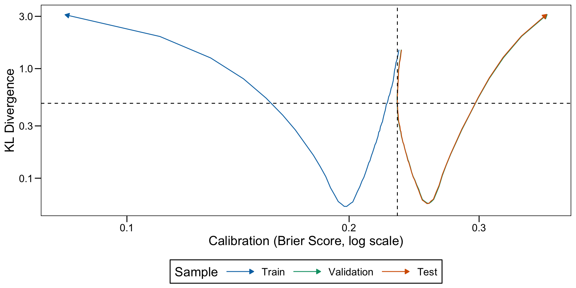
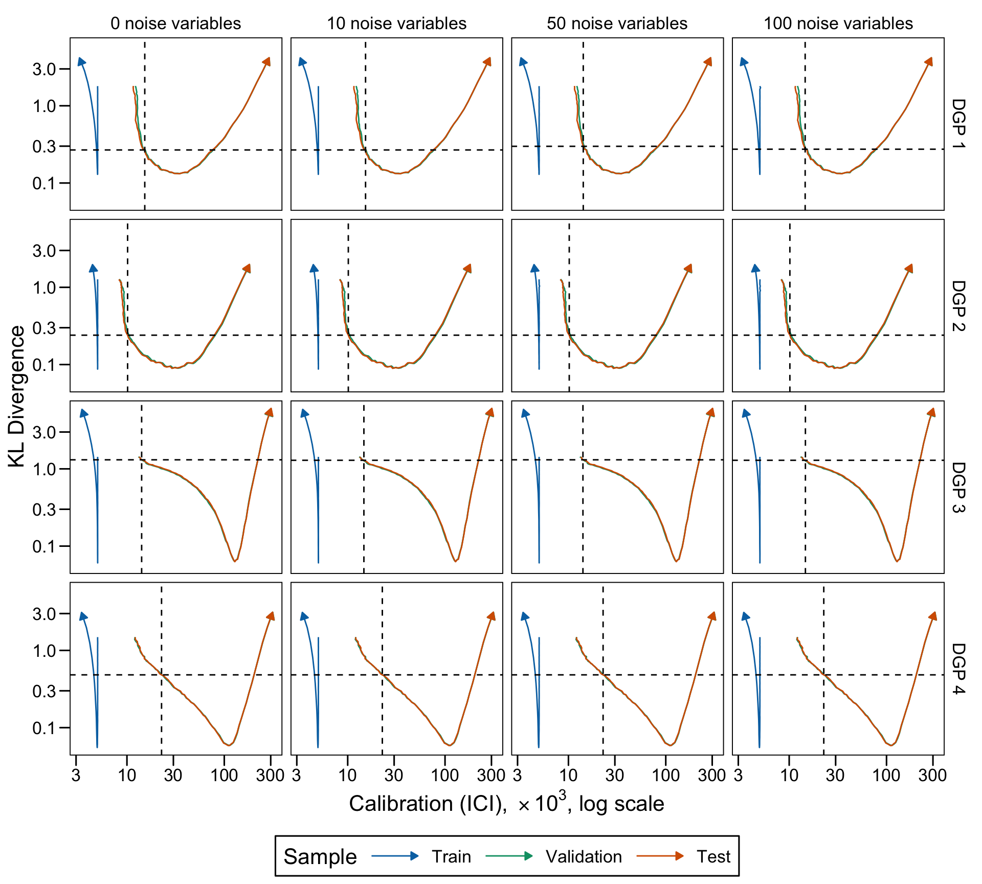
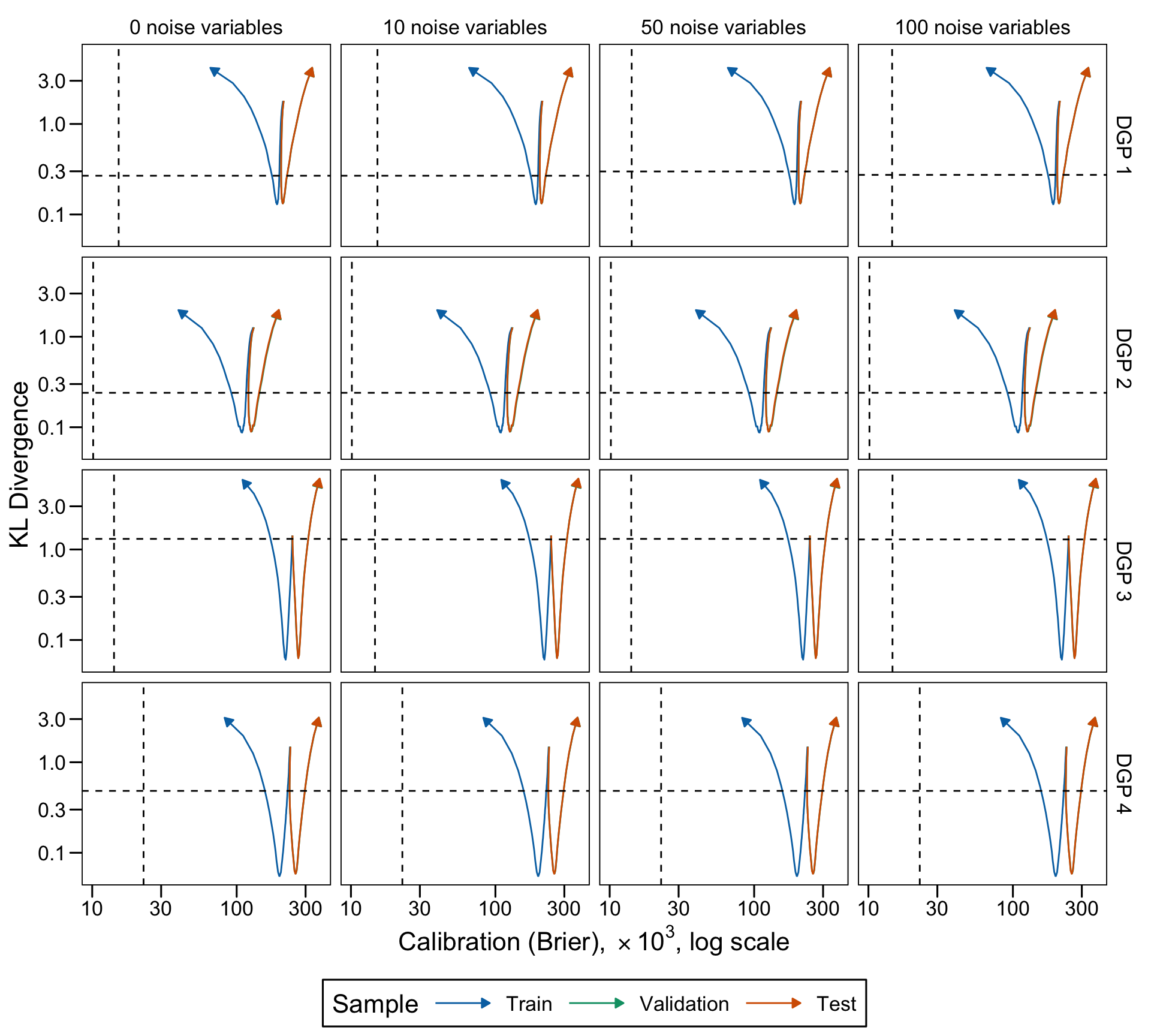
The dashed lines correspond to the values of the KL divergence and the calibration of the forest at which the AUC is the highest among the models of the grid search.

Complexity of a tree and relationship with calibration and divergence of scores to the true probabilities. (DGP 1, 0 noise variables)

Complexity of a tree and relationship with calibration and divergence of scores to the true probabilities. (DGP 1, 10 noise variables)

Complexity of a tree and relationship with calibration and divergence of scores to the true probabilities. (DGP 1, 50 noise variables)

Complexity of a tree and relationship with calibration and divergence of scores to the true probabilities. (DGP 1, 100 noise variables)

Complexity of a tree and relationship with calibration and divergence of scores to the true probabilities. (DGP 2, 0 noise variables)

Complexity of a tree and relationship with calibration and divergence of scores to the true probabilities. (DGP 2, 10 noise variables)

Complexity of a tree and relationship with calibration and divergence of scores to the true probabilities. (DGP 2, 50 noise variables)

Complexity of a tree and relationship with calibration and divergence of scores to the true probabilities. (DGP 2, 100 noise variables)

Complexity of a tree and relationship with calibration and divergence of scores to the true probabilities. (DGP 3, 0 noise variables)

Complexity of a tree and relationship with calibration and divergence of scores to the true probabilities. (DGP 3, 10 noise variables)

Complexity of a tree and relationship with calibration and divergence of scores to the true probabilities. (DGP 3, 50 noise variables)

Complexity of a tree and relationship with calibration and divergence of scores to the true probabilities. (DGP 3, 100 noise variables)

Complexity of a tree and relationship with calibration and divergence of scores to the true probabilities. (DGP 4, 0 noise variables)

Complexity of a tree and relationship with calibration and divergence of scores to the true probabilities. (DGP 4, 10 noise variables)

Complexity of a tree and relationship with calibration and divergence of scores to the true probabilities. (DGP 4, 50 noise variables)

Complexity of a tree and relationship with calibration and divergence of scores to the true probabilities. (DGP 4, 100 noise variables)

Complexity of a tree and relationship with calibration and divergence of scores to the true probabilities. (DGP 1, 0 noise variables, log scale)

Complexity of a tree and relationship with calibration and divergence of scores to the true probabilities. (DGP 1, 10 noise variables, log scale)

Complexity of a tree and relationship with calibration and divergence of scores to the true probabilities. (DGP 1, 50 noise variables, log scale)

Complexity of a tree and relationship with calibration and divergence of scores to the true probabilities. (DGP 1, 100 noise variables, log scale)

Complexity of a tree and relationship with calibration and divergence of scores to the true probabilities. (DGP 2, 0 noise variables, log scale)

Complexity of a tree and relationship with calibration and divergence of scores to the true probabilities. (DGP 2, 10 noise variables, log scale)

Complexity of a tree and relationship with calibration and divergence of scores to the true probabilities. (DGP 2, 50 noise variables, log scale)

Complexity of a tree and relationship with calibration and divergence of scores to the true probabilities. (DGP 2, 100 noise variables, log scale)

Complexity of a tree and relationship with calibration and divergence of scores to the true probabilities. (DGP 3, 0 noise variables, log scale)

Complexity of a tree and relationship with calibration and divergence of scores to the true probabilities. (DGP 3, 10 noise variables, log scale)

Complexity of a tree and relationship with calibration and divergence of scores to the true probabilities. (DGP 3, 50 noise variables, log scale)

Complexity of a tree and relationship with calibration and divergence of scores to the true probabilities. (DGP 3, 100 noise variables, log scale)

Complexity of a tree and relationship with calibration and divergence of scores to the true probabilities. (DGP 4, 0 noise variables, log scale)

Complexity of a tree and relationship with calibration and divergence of scores to the true probabilities. (DGP 4, 10 noise variables, log scale)

Complexity of a tree and relationship with calibration and divergence of scores to the true probabilities. (DGP 4, 50 noise variables, log scale)

Complexity of a tree and relationship with calibration and divergence of scores to the true probabilities. (DGP 4, 100 noise variables, log scale)

We can also put all the scenarios in a single graph.

Codes to create the figure

data_plot <- metrics_trees_all |> 
  group_by(
    sample, scenario, ind
  ) |> 
  summarise(
    KL_20_true_probas = mean(KL_20_true_probas),
    ici = mean(ici),
    brier = mean(brier),
    nb_leaves = mean(nb_leaves),
    auc = mean(AUC),
    .groups = "drop"
  ) |> 
  mutate(
    dgp = case_when(
      scenario %in% 1:4 ~ 1,
      scenario %in% 5:8 ~ 2,
      scenario %in% 9:12 ~ 3,
      scenario %in% 13:16 ~ 4
    ),
    dgp = factor(dgp, levels = 1:4, labels = str_c("DGP ", 1:4)),
    no_noise = c(0, 10, 50, 100)[(scenario-1)%%4 + 1],
    no_noise = factor(
      no_noise, levels = c(0, 10, 50, 100),
      labels = str_c(c(0, 10, 50, 100), " noise variables")
    )
  )


data_plot_max_auc <- 
  data_plot |> 
  filter(sample == "Test") |> 
  group_by(sample, scenario) |> 
  mutate(is_max_auc = auc == max(auc)) |> 
  ungroup() |> 
  filter(is_max_auc == TRUE) |> 
  select(sample, scenario, dgp, no_noise, ici, brier, KL_20_true_probas)

ICI, log scale
Brier, log scale

Codes to create the figure

formatter1000 <- function(x) x*1000

p_ici <- ggplot(
  data = data_plot |> arrange(nb_leaves),
  mapping = aes(
    x = ici, y = KL_20_true_probas
  )
) + 
  geom_path(
    mapping = aes(colour = sample),
    arrow = arrow(type = "closed", ends = "last", 
                  length = unit(0.08, "inches"))
  ) +
  geom_vline(
    data = data_plot_max_auc,
    mapping = aes(xintercept = ici),
    linetype = "dashed"
  ) +
  geom_hline(
    data = data_plot_max_auc,
    mapping = aes(yintercept = KL_20_true_probas),
    linetype = "dashed"
  ) +
  facet_grid(dgp~no_noise) +
  # ggh4x::facet_grid2(dgp~no_noise, scales = "free_y") +
  scale_colour_manual(
    "Sample", values = colour_samples,
    labels = c("Train", "Validation", "Test")) +
  labs(
    x = latex2exp::TeX("Calibration (ICI), $\\times 10^{3}$, log scale"), 
    y = "KL Divergence"
  ) +
  theme_paper() +
  theme(legend.key.width = unit(1.5, "cm")) +
  scale_x_log10(labels = formatter1000) + scale_y_log10()

ggsave(p_ici, file = "figures/trees-kl-calib-ici-leaves-all.pdf",
       width = 10, height = 8)

p_ici

Figure 5.2: KL Divergence and Calibration (ICI) across increasing average number of leaves in the trees (log scales)

Codes to create the figure

formatter1000 <- function(x) x*1000

p_brier <- ggplot(
  data = data_plot |> arrange(nb_leaves),
  mapping = aes(
    x = brier, y = KL_20_true_probas
  )
) + 
  geom_path(
    mapping = aes(colour = sample),
    arrow = arrow(type = "closed", ends = "last", 
                  length = unit(0.08, "inches"))
  ) +
  geom_vline(
    data = data_plot_max_auc,
    mapping = aes(xintercept = ici),
    linetype = "dashed"
  ) +
  geom_hline(
    data = data_plot_max_auc,
    mapping = aes(yintercept = KL_20_true_probas),
    linetype = "dashed"
  ) +
  facet_grid(dgp~no_noise) +
  scale_colour_manual(
    "Sample", values = colour_samples,
    labels = c("Train", "Validation", "Test")) +
  labs(
    x = latex2exp::TeX("Calibration (Brier), $\\times 10^{3}$, log scale"), 
    y = "KL Divergence"
  ) +
  theme_paper() +
  theme(legend.key.width = unit(1.5, "cm")) +
  scale_x_log10(labels = formatter1000) + scale_y_log10()

ggsave(p_brier, file = "figures/trees-kl-calib-brier-leaves-all.pdf",
       width = 10, height = 8)

p_brier

Figure 5.3: KL Divergence and Calibration (ICI) across increasing average number of leaves in the trees (log scales)