2  Targeted Distribution

Note

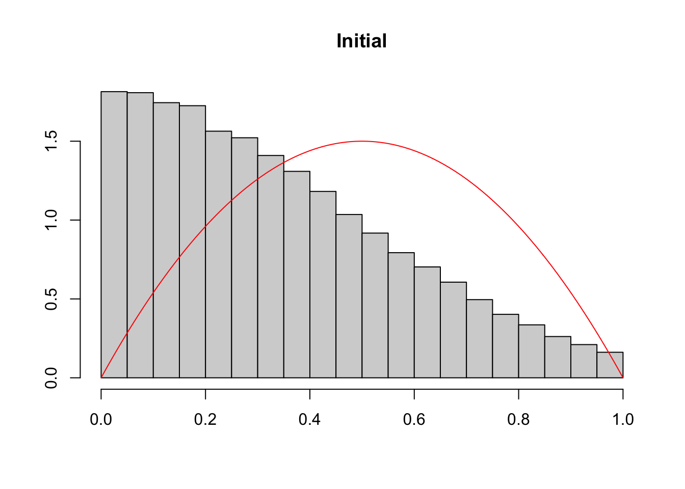
In this chapter, we provide some codes to simulate a dataset with a binary variable for which the underlying probability follows a targeted distribution. We consider here, as an example, that we would like the true probabilities to follow a Beta(2,2) distribution.

Code Availability

The functions used to subsample from a dataset so that the true probabilities in that subsample follows a target distribution are saved in the functions/subsample_target_distrib.r.

library(ks)
library(tidyverse)

── Attaching core tidyverse packages ──────────────────────── tidyverse 2.0.0 ──
✔ dplyr     1.1.4     ✔ readr     2.1.5
✔ forcats   1.0.0     ✔ stringr   1.5.1
✔ ggplot2   3.5.1     ✔ tibble    3.2.1
✔ lubridate 1.9.3     ✔ tidyr     1.3.1
✔ purrr     1.0.2     
── Conflicts ────────────────────────────────────────── tidyverse_conflicts() ──
✖ dplyr::filter() masks stats::filter()
✖ dplyr::lag()    masks stats::lag()
ℹ Use the conflicted package (<http://conflicted.r-lib.org/>) to force all conflicts to become errors

2.1 Algorithm

In our generated sample, \(\mathcal{D}=\{(\boldsymbol{x}_i,y_i,{s}_i),i\in\{1,\cdots,n\}\}\), let \(\widehat{f}\) denote the (empirical) density of scores. For the various scenarios, suppose that we want a specific distribution for the scores, denoted \(g\) (uniform, Beta, etc.). A classical idea is to use ‘’rejection sampling’’ techniques to create a subsample of the dataset. Set \[ c = \sup_{s\in(0,1)} \frac{\widehat{f}(s)}{g(s)} \leq \infty. \] If \(c\) is finite, and not too large, we can use the standard rejection technique, described in Algorithm 2.1. In a nutshell, point \(i\) is kept with probability \((cg(s_i))^{-1}\widehat{f}(s_i)\).

\begin{algorithm} \caption{Subsample a dataset so that the distribution of scores has density $g$ (Rejection, $c$ small)} \begin{algorithmic} \Require $\mathcal{D}=\{(\boldsymbol{x}_i,y_i,{s}_i),i\in\{1,\cdots,n\}\}$ and $g$ (target density) \State $\mathcal{I} \gets ,i\in\{1,\cdots,n\}$ \State $\widehat{f} \gets$ density of $\{({s}_i),i\in\mathcal{I}\}$, using Chen (1999) \State $c = \displaystyle\sup_{s\in(0,1)} \frac{\widehat{f}(s)}{g(s)} \gets \max_{i=1,\cdots,n}\displaystyle\frac{\widehat{f}(s_i)}{g(s_i)} $ \For{$i\in\{1,\cdots,n\}$} \State $U \gets \mathcal{U}([0,1])$ \If{$\displaystyle U > \frac{\widehat{f}(s_i)}{c\,g(s_i)}$} \State $\mathcal{I} \gets \mathcal{I}\backslash\{i\}$ , i.e. ``reject" \EndIf \EndFor \State $s\mathcal{D}=\{(\boldsymbol{x}_i,y_i,{s}_i),i\in\mathcal{I}\}$ \end{algorithmic} \end{algorithm}

Note: the reference mentioned: Chen (1999)

If \(c\) is too large, we use an iterative algorithm, described in Algorithm 2.2, inspired by Rumbell et al. (2023) (alternative options could be the ‘’Empirical Supremum Rejection Sampling’’ introduced in Caffo, Booth, and Davison (2002), for instance)

\begin{algorithm} \caption{Subsample a dataset so that the distribution of scores has density $g$ (Iterative Rejection, $c$ large)} \begin{algorithmic} \Require $\mathcal{D}=\{(\boldsymbol{x}_i,y_i,{s}_i),i\in\{1,\cdots,n\}\}$, $\epsilon>0$ and $g$ (target density) \State $\mathcal{I} \gets \{1,\cdots,n\}$ \State $\widehat{f} \gets$ density of $\{({s}_i),i\in\mathcal{I}\}$, using Chen (1999) \State $d \gets \|\widehat{F}-G\|_{\infty}$ (Kolmogorov-Smirnov distance) \While{$d>\epsilon$} \State $\mathcal{J} \gets \mathcal{I}$ \For{$i\in\mathcal{I}$} \State $U \gets \mathcal{U}([0,1])$ \If{$\displaystyle U>\frac{\widehat{f}(s_i)}{g(s_i)}$} \State $\mathcal{J} \gets \mathcal{J}\backslash\{i\}$ , i.e. 'reject' observation $i$ \EndIf \EndFor \State $\mathcal{I} \gets \mathcal{J}$ \State $\widehat{f} \gets$ density of $\{({s}_i),i\in\mathcal{I}\}$ \State $d \gets \|\widehat{F}-G\|_{\infty}$ \EndWhile \State $s\mathcal{D}=\{(\boldsymbol{x}_i,y_i,{s}_i),i\in\mathcal{I}\}$ \end{algorithmic} \end{algorithm}

To implement this, we define the subset_target() function.

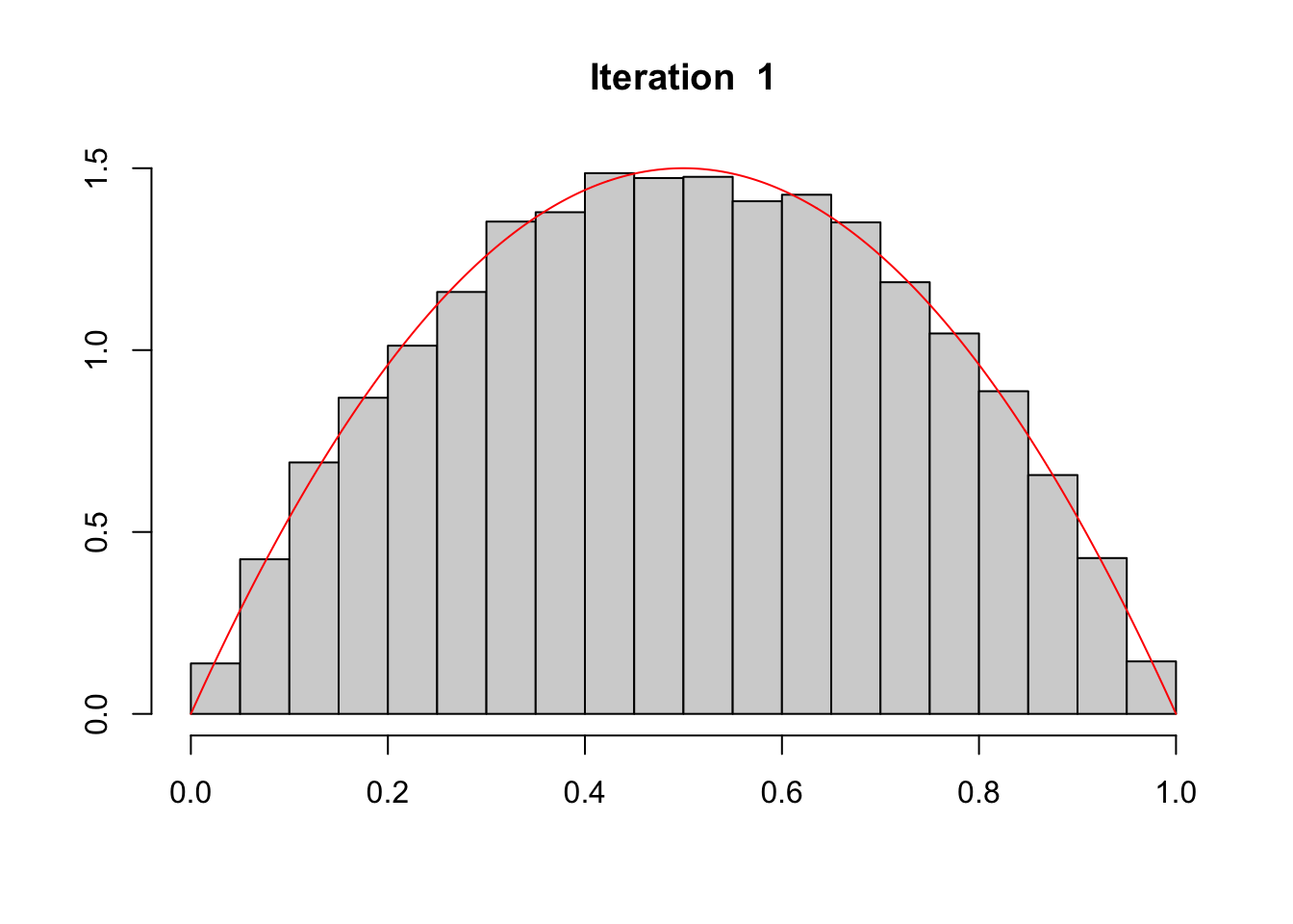
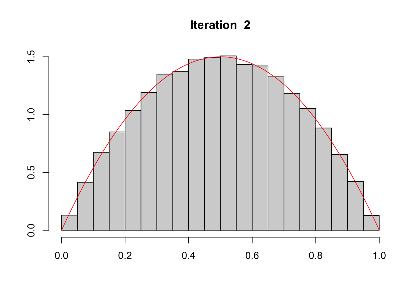
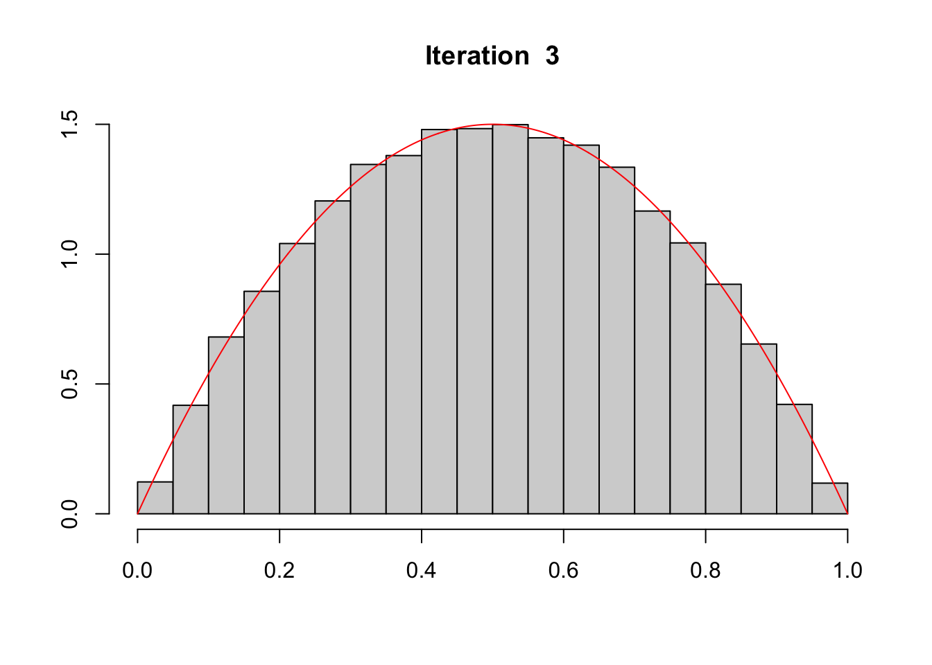
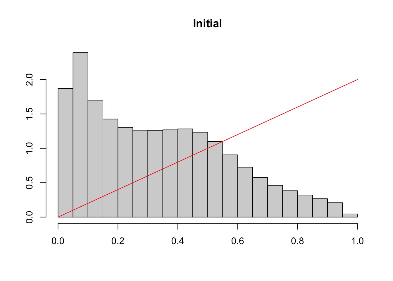
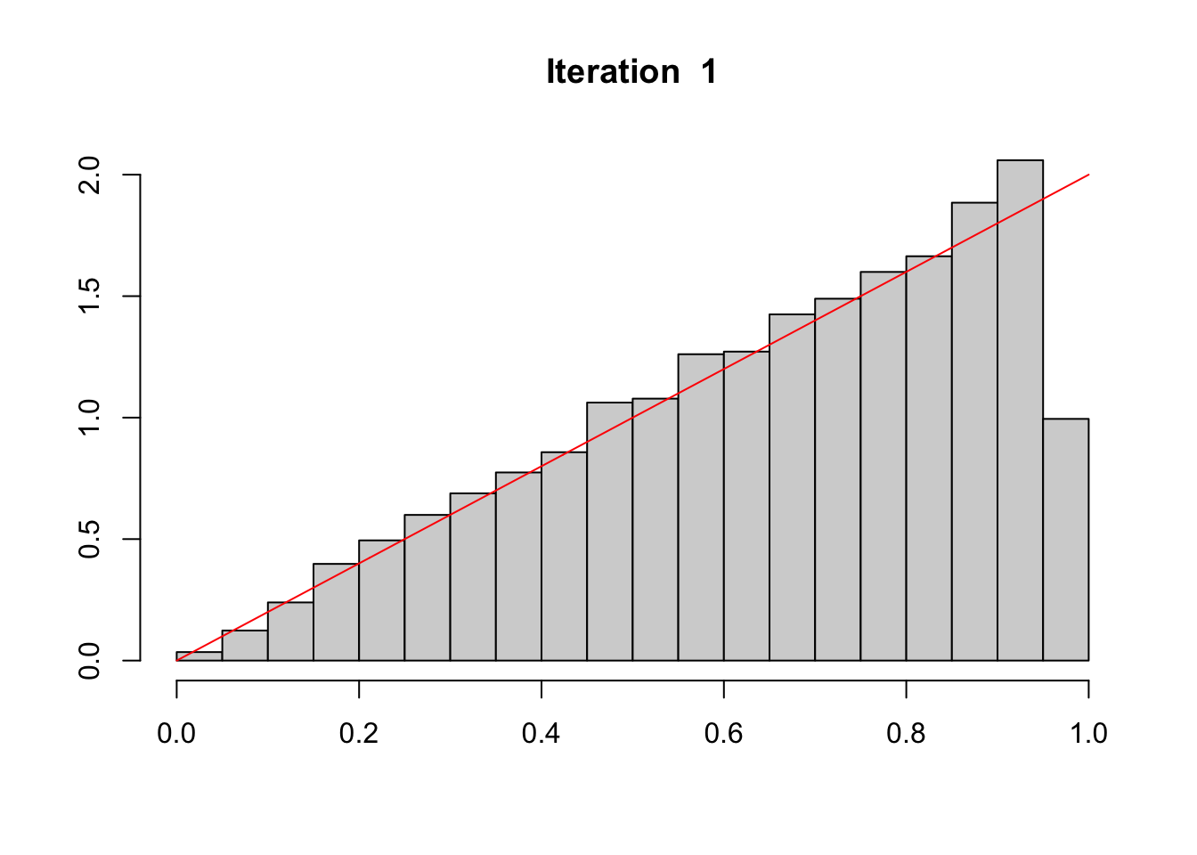
#' @param data dataset
#' @param score_name name of the column in data that contains the scores
#' @param target_fun target distribution function.
#' @param iter number of iterations.
#' @param draw if TRUE (default) the distribution of scores (gray bars) and the
#'  target distribution (in red) are plotted at each iteration.
#' @seed if not `NULL`, seed to use
#' @param data dataset
#' @param probs_name name of the column in data that contains the observed
#'  probabilities
#' @param target_fun target distribution function.
#' @param iter number of iterations.
#' @param draw if TRUE (default) the distribution of scores (gray bars) and the
#'  target distribution (in red) are plotted at each iteration.
#' @seed if not `NULL`, seed to use
#' @param verbose if `FALSE`, size of subsamplings at each iteration and KS test
#'  results are hiddent
subset_target <- function(data,
                          probs_name,
                          target_fun = function(x) dbeta(x,2,2),
                          iter = 1,
                          draw = TRUE,
                          seed = NULL,
                          verbose = TRUE){
  select <- rep(nrow(data),iter + 1)
  if (!is.null(seed)) set.seed(seed)

  # Get the scores from the dataset
  probs_01 <- data |> pull(!!probs_name)
  if (verbose == TRUE) cat("1) Size ...... ", nrow(data), "\n", sep = "")

  # Kolmogorov-Smirnov Test
  fun <- Vectorize(function(x) integrate(target_fun, 0, x)$value)
  K <- ks.test(probs_01, fun)

  if (verbose) {
    cat("1)  ks ............ ", K$statistic, "\n", sep = "")
    cat("1)  (pvalue) ...... ", K$p.value, "\n", sep = "")
  }

  if (draw) {
    # Histogram of scores (gray) and target distribution (red)
    hist(probs_01,probability = TRUE, xlab = "", ylab = "", main = "Initial")
    val_x <- seq(0,1,length = 601)
    lines(val_x,target_fun(val_x), col = "red")
  }

  data_subset <- data

  for (k in 1:iter) {
    n <- nrow(data_subset)
    initial_density <- kde(x = probs_01, eval.points = probs_01)
    # Probability to include each observation in the current subset
    prob_acceptation <- target_fun(probs_01) / initial_density$estimate
    prob_acceptation <- pmin(prob_acceptation / max(prob_acceptation), 1)
    # For each scores from the current data subset, decide whether or not to
    # include it based on a random draw from a Ber(prob_acceptation)
    index_acceptation <- rbinom(n, size = 1, prob = prob_acceptation)
    # Use this index to keep only the selected data
    data_subset <- data_subset[which(index_acceptation ==1 ), ]
    select[k + 1] <- nrow(data_subset)
    probs_01 <- data_subset |> pull(!!probs_name)
    if (verbose == TRUE)
      cat(k + 1, ") Size ...... ", nrow(data_subset), "\n", sep = "")
    # Kolmogorov-Smirnov Test
    K <- ks.test(probs_01, fun)
    if (verbose) {
      cat(k + 1, ")   ks ............ ", K$statistic, "\n", sep = "")
      cat(k + 1, ")   (pvalue) ...... ", K$p.value, "\n", sep = "")
    }
    if (draw) {
      hist(
        probs_01, probability = TRUE, xlab = "", ylab = "",
        main = paste("Iteration ", k)
      )
      val_x <- seq(0, 1, length = 601)
      lines(val_x, target_fun(val_x), col = "red")
    }
  }
  data_subset
}

2.2 First Example

Let us begin with generating some binary data, using a linear predictor for the true probability.

n <- 1e5 # Number of obs.
# Covariates
x1 <- rnorm(n)
x2 <- rnorm(n)
# True probabilities
p <- function(x1, x2) .4 * x1 - .2*x2
# Observed event
y <- rnorm(n,p(x1, x2), .4)
tb <- tibble(y = y, x1 = x1, x2 = x2)

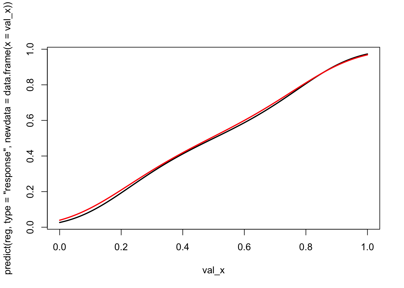
Let us consider a linear model to predict the observed event:

reg <- lm(y ~ x1 + x2, data = tb)
scores <- predict(reg)
tb$scores <- scores

Keeping only scores between 0 and 1 (would not need to do so for glm)

tb_01 <- tb[(scores > 0) & (scores < 1), ]
data <- tb_01

B <- subset_target(data = data, probs_name = "scores", iter = 4)

1) Size ...... 48913
1)  ks ............ 0.2978291
1)  (pvalue) ...... 0

2) Size ...... 17882
2)   ks ............ 0.00497645
2)   (pvalue) ...... 0.767677

3) Size ...... 17213
3)   ks ............ 0.002497988
3)   (pvalue) ...... 0.9999214

4) Size ...... 16947
4)   ks ............ 0.00244163
4)   (pvalue) ...... 0.9999608

5) Size ...... 16519
5)   ks ............ 0.002052978
5)   (pvalue) ...... 0.9999998

Let us consider another example.

library(splines)

2.3 Second Examplle

We generate another dataset.

n <- 1e6
x <- rbeta(n, 1, 2)
y <- rbinom(n, size = 1, prob = x)
base <- tibble(
  x = x,
  y = y,
  id = 1:n
)

Let us assume that the scores are estimated using a logistic model.

reg <- glm(y ~ bs(x), data = base, family = binomial)
base$scores <- predict(reg, type = "response")

Let us further assume that we want the scores to be distributed according to a Beta(2,1).

B <- subset_target(
  data = base, 
  probs_name = "scores", 
  iter = 1, 
  target_fun = function(x) dbeta(x,2,1)
)

1) Size ...... 1000000

Warning in ks.test.default(probs_01, fun): ties should not be present for the
one-sample Kolmogorov-Smirnov test

1)  ks ............ 0.5034374
1)  (pvalue) ...... 0

2) Size ...... 7439
2)   ks ............ 0.05460811
2)   (pvalue) ...... 1.07831e-19

We check the new observations:

reg2 <- glm(y ~ bs(x), data = B, family = binomial)

val_x <- seq(0, 1, length = 601)
plot(
  val_x,
  predict(reg, type = "response", newdata = data.frame(x = val_x)),
  type = "l", lwd = 2
)

Warning in bs(x, degree = 3L, knots = numeric(0), Boundary.knots =
c(6.39120525304657e-07, : some 'x' values beyond boundary knots may cause
ill-conditioned bases

lines(
  val_x,
  predict(reg2, type = "response", newdata = data.frame(x = val_x)),
  type = "l", lwd = 2, col = "red"
)

Warning in bs(x, degree = 3L, knots = numeric(0), Boundary.knots =
c(0.00380140183344815, : some 'x' values beyond boundary knots may cause
ill-conditioned bases

Caffo, Brian S, James G Booth, and AC Davison. 2002. “Empirical Supremum Rejection Sampling.” Biometrika 89 (4): 745–54.

Chen, Song Xi. 1999. “Beta Kernel Estimators for Density Functions.” Computational Statistics & Data Analysis 31 (2): 131–45.

Rumbell, Timothy, Jaimit Parikh, James Kozloski, and Viatcheslav Gurev. 2023. “Novel and Flexible Parameter Estimation Methods for Data-Consistent Inversion in Mechanistic Modelling.” Royal Society Open Science 10 (11): 230668.