9 Counterfactuals: comparison

Objectives

This chapter compares the different methods used to create counterfactuals by examining the impacts on the new predictions made by the classifiers (aware and unaware).

Display the setting codes

# Required packages----
library(tidyverse)
library(fairadapt)

# Graphs----
font_main = font_title = 'Times New Roman'
extrafont::loadfonts(quiet = T)
face_text='plain'
face_title='plain'
size_title = 14
size_text = 11
legend_size = 11

global_theme <- function() {
  theme_minimal() %+replace%
    theme(
      text = element_text(family = font_main, size = size_text, face = face_text),
      legend.text = element_text(family = font_main, size = legend_size),
      axis.text = element_text(size = size_text, face = face_text), 
      plot.title = element_text(
        family = font_title, 
        size = size_title, 
        hjust = 0.5
      ),
      plot.subtitle = element_text(hjust = 0.5)
    )
}

# Seed
set.seed(2025)

source("../functions/utils.R")

9.1 Load Data and Classifier

We load the dataset where the sensitive attribute ((S)) is the race, obtained Chapter 4.3:

load("../data/df_race.rda")

Counterfactuals constructed with fairadapt and predictions by the classifiers (see Chapter 6):

load("../data/counterfactuals_aware_fpt.rda")
load("../data/counterfactuals_unaware_fpt.rda")

Counterfactuals constructed with multivariate optimal transport and predictions by the classifiers (see Chapter 7):

load("../data/counterfactuals_aware_ot.rda")
load("../data/counterfactuals_unaware_ot.rda")

Counterfactuals constructed with sequential transport and predictions by the classifiers (see Chapter 8):

load("../data/counterfactuals_aware_seq_black.rda")
load("../data/counterfactuals_unaware_seq_black.rda")

We also need the predictions made by the classifier (see Chapter 5):

# Predictions on train/test sets
load("../data/pred_aware.rda")
load("../data/pred_unaware.rda")
# Predictions on the factuals, on the whole dataset
load("../data/pred_aware_all.rda")
load("../data/pred_unaware_all.rda")

We create a tibble with the factuals and the predictions by the aware model, an another with the predictions by the unaware model:

factuals_aware <- tibble(
  S = df_race$S,
  X1 = df_race$X1,
  X2 = df_race$X2,
  pred = pred_aware_all,
  type = "factual"
)

factuals_unaware <- tibble(
  S = df_race$S,
  X1 = df_race$X1,
  X2 = df_race$X2,
  pred = pred_unaware_all,
  type = "factual"
)

9.2 Comparison

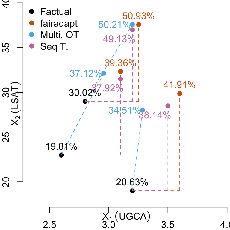
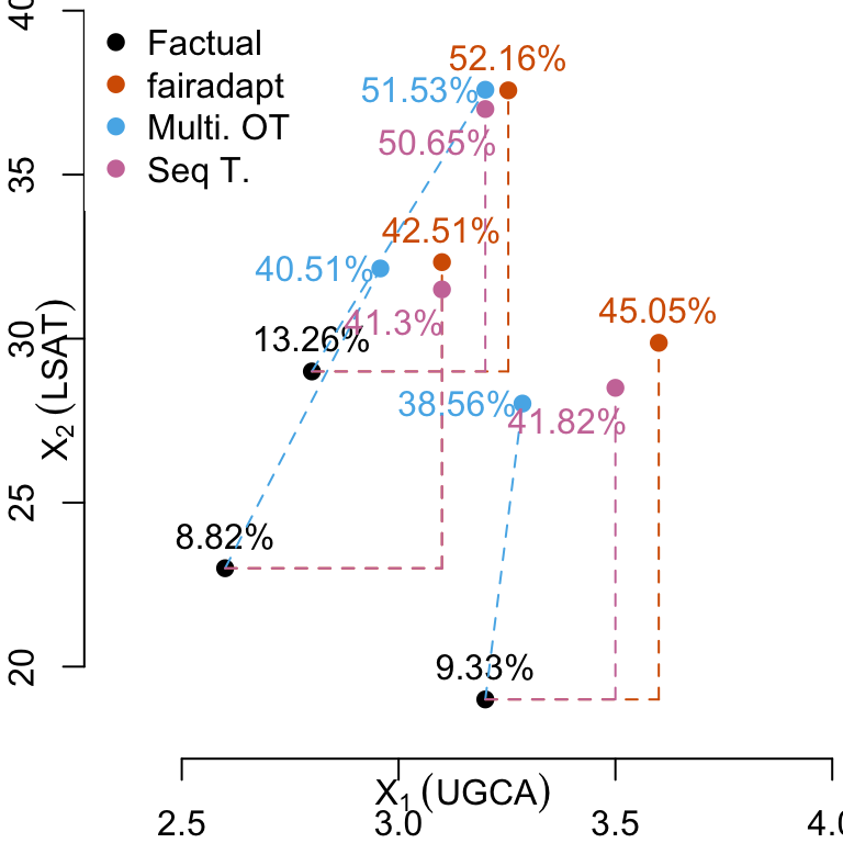
Let us focus on the first three Black individuals from the dataset. We will compare the predicted values by the classifier (see Chapter 5) made using the observed characteristics, and the changes in the predictions when using counterfactuals. We use the three types of counterfactuals explored in the previous chapters.

Unaware Model
Aware Model

tb_unaware <- 
  factuals_unaware |> mutate(id = row_number(), counterfactual = "none") |> 
  # Fairadapt
  bind_rows(
    counterfactuals_unaware_fpt |> 
      mutate(id = row_number(), counterfactual = "fpt")
  ) |> 
  # Multivariate optimal transport
  bind_rows(
    counterfactuals_unaware_ot |> mutate(id = row_number(), counterfactual = "ot")
  ) |> 
  # Sequential transport
  bind_rows(
    counterfactuals_unaware_seq_black |> mutate(counterfactual = "seq")
  )

tb_indiv_unaware <- 
  tb_unaware |> 
  filter(id %in% counterfactuals_unaware_seq_black$id[1:3])

tb_indiv_unaware

# A tibble: 12 × 7
   S        X1    X2  pred type              id counterfactual
   <chr> <dbl> <dbl> <dbl> <chr>          <int> <chr>         
 1 Black  2.8   29   0.300 factual           24 none          
 2 Black  3.2   19   0.206 factual           40 none          
 3 Black  2.6   23   0.198 factual           51 none          
 4 White  3.25  37.6 0.509 counterfactual    24 fpt           
 5 White  3.6   29.9 0.419 counterfactual    40 fpt           
 6 White  3.1   32.3 0.394 counterfactual    51 fpt           
 7 White  3.20  37.6 0.502 counterfactual    24 ot            
 8 White  3.29  28.0 0.345 counterfactual    40 ot            
 9 White  2.96  32.1 0.371 counterfactual    51 ot            
10 White  3.2   37   0.491 counterfactual    24 seq           
11 White  3.5   28.5 0.381 counterfactual    40 seq           
12 White  3.1   31.5 0.379 counterfactual    51 seq

tb_aware <- 
  factuals_aware |> mutate(id = row_number(), counterfactual = "none") |> 
  # Fairadapt
  bind_rows(
    counterfactuals_aware_fpt |> 
      mutate(id = row_number(), counterfactual = "fpt")
  ) |> 
  # Multivariate optimal transport
  bind_rows(
    counterfactuals_aware_ot |> mutate(id = row_number(), counterfactual = "ot")
  ) |> 
  # Sequential transport
  bind_rows(
    counterfactuals_aware_seq_black |> mutate(counterfactual = "seq")
  ) 
  
tb_indiv_aware <- 
  tb_aware |> 
  filter(id %in% counterfactuals_aware_seq_black$id[1:3])

tb_indiv_aware

# A tibble: 12 × 7
   S        X1    X2   pred type              id counterfactual
   <chr> <dbl> <dbl>  <dbl> <chr>          <int> <chr>         
 1 Black  2.8   29   0.133  factual           24 none          
 2 Black  3.2   19   0.0933 factual           40 none          
 3 Black  2.6   23   0.0882 factual           51 none          
 4 White  3.25  37.6 0.522  counterfactual    24 fpt           
 5 White  3.6   29.9 0.451  counterfactual    40 fpt           
 6 White  3.1   32.3 0.425  counterfactual    51 fpt           
 7 White  3.20  37.6 0.515  counterfactual    24 ot            
 8 White  3.29  28.0 0.386  counterfactual    40 ot            
 9 White  2.96  32.1 0.405  counterfactual    51 ot            
10 White  3.2   37   0.507  counterfactual    24 seq           
11 White  3.5   28.5 0.418  counterfactual    40 seq           
12 White  3.1   31.5 0.413  counterfactual    51 seq

Unaware Model
Aware Model

Code

par(mar = c(2, 2, 0, 0))
# Initial characteristics with the unaware model
tb_indiv_unaware_factual <- 
  tb_indiv_unaware |> filter(type == "factual")
colour_factual <- "black"
colour_fpt <- "#D55E00"
colour_ot <- "#56B4E9"
colour_seq <- "#CC79A7"
colours_all <- c(
  "Factual" = colour_factual,
  "fairadapt" = colour_fpt,
  "Multi. OT" = colour_ot,
  "Seq T." = colour_seq
)
range_x1 <- range(tb_indiv_unaware$X1)
expansion_amount_x1 <- .1*range_x1
range_x2 <- range(tb_indiv_unaware$X2)
expansion_amount_x2 <- .05*range_x2

plot(
  x = tb_indiv_unaware_factual$X1,
  y = tb_indiv_unaware_factual$X2,
  col = colour_factual,
  # xlab = "X1 (UGPA)", ylab = "X2 (LSAT)",
  xlab = "", ylab = "",
  xlim = c(range_x1[1] - expansion_amount_x1[1], range_x1[2] + expansion_amount_x1[2]),
  ylim = c(range_x2[1] - expansion_amount_x2[1], range_x2[2] + expansion_amount_x2[2]),
  pch = 19,
  axes = FALSE
)
axis(1)
mtext(expression(X[1]~(UGCA)), side = 1, padj = .5)
axis(2)
mtext(expression(X[2]~(LSAT)), side = 2, padj = 0)
text(
  x = tb_indiv_unaware_factual$X1, 
  y = tb_indiv_unaware_factual$X2 + 1,
  paste0(round(100*tb_indiv_unaware_factual$pred, 2), "%"),
  col = colour_factual
)
# Transported characteristics with fairadapt
tb_indiv_unaware_fpt <- 
  tb_indiv_unaware |> filter(counterfactual == "fpt")
points(
  x = tb_indiv_unaware_fpt$X1,
  y = tb_indiv_unaware_fpt$X2,
  col = colour_fpt,
  xlab = "X1", ylab = "X2",
  pch = 19
)
# x1 then x2
segments(
  x0 = tb_indiv_unaware_factual$X1, 
  y0 = tb_indiv_unaware_factual$X2,
  x1 = tb_indiv_unaware_fpt$X1, 
  y1 = tb_indiv_unaware_factual$X2, 
  col = colour_fpt,
  lty = 2
)
segments(
  x0 = tb_indiv_unaware_fpt$X1, 
  y0 = tb_indiv_unaware_factual$X2,
  x1 = tb_indiv_unaware_fpt$X1, 
  y1 = tb_indiv_unaware_fpt$X2, 
  col = colour_fpt,
  lty = 2
)
text(
  x = tb_indiv_unaware_fpt$X1, 
  y = tb_indiv_unaware_fpt$X2 + 1,
  paste0(round(100*tb_indiv_unaware_fpt$pred, 2), "%"),
  col = colour_fpt
)
# Transported characteristics with OT
tb_indiv_unaware_ot <- 
  tb_indiv_unaware |> filter(counterfactual == "ot")
points(
  x = tb_indiv_unaware_ot$X1,
  y = tb_indiv_unaware_ot$X2,
  col = colour_ot,
  xlab = "X1", ylab = "X2",
  pch = 19
)
# x1 then x2
segments(
  x0 = tb_indiv_unaware_factual$X1, 
  y0 = tb_indiv_unaware_factual$X2,
  x1 = tb_indiv_unaware_ot$X1, 
  y1 = tb_indiv_unaware_ot$X2, 
  col = colour_ot,
  lty = 2
)
text(
  x = tb_indiv_unaware_ot$X1 - .15, 
  y = tb_indiv_unaware_ot$X2,
  paste0(round(100*tb_indiv_unaware_ot$pred, 2), "%"),
  col = colour_ot
)

# Transported characteristics with Sequential transport
tb_indiv_unaware_seq <- 
  tb_indiv_unaware |> filter(counterfactual == "seq")
points(
  x = tb_indiv_unaware_seq$X1,
  y = tb_indiv_unaware_seq$X2,
  col = colour_seq,
  xlab = "X1", ylab = "X2",
  pch = 19
)
# x1 then x2
segments(
  x0 = tb_indiv_unaware_factual$X1, 
  y0 = tb_indiv_unaware_factual$X2,
  x1 = tb_indiv_unaware_seq$X1, 
  y1 = tb_indiv_unaware_factual$X2, 
  col = colour_seq,
  lty = 2
)
segments(
  x0 = tb_indiv_unaware_seq$X1, 
  y0 = tb_indiv_unaware_factual$X2,
  x1 = tb_indiv_unaware_seq$X1, 
  y1 = tb_indiv_unaware_seq$X2, 
  col = colour_seq,
  lty = 2
)
text(
  x = tb_indiv_unaware_seq$X1 - .11, 
  y = tb_indiv_unaware_seq$X2 - 1,
  paste0(round(100*tb_indiv_unaware_seq$pred, 2), "%"),
  col = colour_seq
)
legend(
  "topleft", 
  pch = 19, col = colours_all, legend = names(colours_all),
  box.lty=0
)

Figure 9.1: Predictions by the unaware model for three Black individuals.

Code

par(mar = c(2, 2, 0, 0))
# Initial characteristics with the aware model
tb_indiv_aware_factual <- 
  tb_indiv_aware |> filter(type == "factual")

range_x1 <- range(tb_indiv_aware$X1)
expansion_amount_x1 <- .1*range_x1
range_x2 <- range(tb_indiv_aware$X2)
expansion_amount_x2 <- .05*range_x2

plot(
  x = tb_indiv_aware_factual$X1,
  y = tb_indiv_aware_factual$X2,
  col = colour_factual,
  xlab = "", ylab = "",
  # xlab = "X1 (UGPA)", ylab = "X2 (LSAT)",
  xlim = c(range_x1[1] - expansion_amount_x1[1], range_x1[2] + expansion_amount_x1[2]),
  ylim = c(range_x2[1] - expansion_amount_x2[1], range_x2[2] + expansion_amount_x2[2]),
  pch = 19,
  axes = FALSE
)
axis(1)
mtext(expression(X[1]~(UGCA)), side = 1, padj = .5)
axis(2)
mtext(expression(X[2]~(LSAT)), side = 2, padj = 0)
text(
  x = tb_indiv_aware_factual$X1, 
  y = tb_indiv_aware_factual$X2 + 1,
  paste0(round(100*tb_indiv_aware_factual$pred, 2), "%"),
  col = colour_factual
)
# Transported characteristics with fairadapt
tb_indiv_aware_fpt <- 
  tb_indiv_aware |> filter(counterfactual == "fpt")
points(
  x = tb_indiv_aware_fpt$X1,
  y = tb_indiv_aware_fpt$X2,
  col = colour_fpt,
  xlab = "X1", ylab = "X2",
  pch = 19
)
# x1 then x2
segments(
  x0 = tb_indiv_aware_factual$X1, 
  y0 = tb_indiv_aware_factual$X2,
  x1 = tb_indiv_aware_fpt$X1, 
  y1 = tb_indiv_aware_factual$X2, 
  col = colour_fpt,
  lty = 2
)
segments(
  x0 = tb_indiv_aware_fpt$X1, 
  y0 = tb_indiv_aware_factual$X2,
  x1 = tb_indiv_aware_fpt$X1, 
  y1 = tb_indiv_aware_fpt$X2, 
  col = colour_fpt,
  lty = 2
)
text(
  x = tb_indiv_aware_fpt$X1, 
  y = tb_indiv_aware_fpt$X2 + 1,
  paste0(round(100*tb_indiv_aware_fpt$pred, 2), "%"),
  col = colour_fpt
)
# Transported characteristics with OT
tb_indiv_aware_ot <- 
  tb_indiv_aware |> filter(counterfactual == "ot")
points(
  x = tb_indiv_aware_ot$X1,
  y = tb_indiv_aware_ot$X2,
  col = colour_ot,
  xlab = "X1", ylab = "X2",
  pch = 19
)
# x1 then x2
segments(
  x0 = tb_indiv_aware_factual$X1, 
  y0 = tb_indiv_aware_factual$X2,
  x1 = tb_indiv_aware_ot$X1, 
  y1 = tb_indiv_aware_ot$X2, 
  col = colour_ot,
  lty = 2
)
text(
  x = tb_indiv_aware_ot$X1 - .15, 
  y = tb_indiv_aware_ot$X2,
  paste0(round(100*tb_indiv_aware_ot$pred, 2), "%"),
  col = colour_ot
)

# Transported characteristics with Sequential transport
tb_indiv_aware_seq <- 
  tb_indiv_aware |> filter(counterfactual == "seq")
points(
  x = tb_indiv_aware_seq$X1,
  y = tb_indiv_aware_seq$X2,
  col = colour_seq,
  xlab = "X1", ylab = "X2",
  pch = 19
)
# x1 then x2
segments(
  x0 = tb_indiv_aware_factual$X1, 
  y0 = tb_indiv_aware_factual$X2,
  x1 = tb_indiv_aware_seq$X1, 
  y1 = tb_indiv_aware_factual$X2, 
  col = colour_seq,
  lty = 2
)
segments(
  x0 = tb_indiv_aware_seq$X1, 
  y0 = tb_indiv_aware_factual$X2,
  x1 = tb_indiv_aware_seq$X1, 
  y1 = tb_indiv_aware_seq$X2, 
  col = colour_seq,
  lty = 2
)
text(
  x = tb_indiv_aware_seq$X1 - .11, 
  y = tb_indiv_aware_seq$X2 - 1,
  paste0(round(100*tb_indiv_aware_seq$pred, 2), "%"),
  col = colour_seq
)
legend(
  "topleft", 
  pch = 19, col = colours_all, legend = names(colours_all),
  box.lty=0
)

Figure 9.2: Predictions by the aware model for three Black individuals.

9.3 Densities

Let us now compare the densities of the predicted values.

colours <- c(
  "0" = "#5BBCD6",
  "1" = "#FF0000",
  "A" = "#00A08A",
  "B" = "#F2AD00",
  "with" = "#046C9A",
  "without" = "#C93312",
  "2" = "#0B775E"
)

Unaware model
Aware model

Code

# Factuals
colours_all <- c(
  "Factual Black" = colours[["A"]],
  "Factual White" = colours[["B"]],
  "fairadapt" = colour_fpt,
  "OT" = colour_ot,
  "Seq T." = colour_seq
)

# Factuals
tb_unaware_factuals <- tb_unaware |> 
  filter(counterfactual == "none")
# Predicted values
pred_unaware_factuals_black <- tb_unaware_factuals |> filter(S == "Black") |> pull("pred")
pred_unaware_factuals_white <- tb_unaware_factuals |> filter(S == "White") |> pull("pred")
# Estimated densities
d_unaware_factuals_black <- density(pred_unaware_factuals_black)
d_unaware_factuals_white <- density(pred_unaware_factuals_white)

par(mfrow = c(3, 1), mar = c(2, 2, 0, 0))
x_lim <- c(0, .8)
y_lim <- c(0, 8)

# plot(
#   d_unaware_factuals_black,
#   main = "Factuals", xlab = "", ylab = "",
#   axes = FALSE, col = NA,
#   xlim = x_lim
# )
# axis(1)
# axis(2)
# polygon(d_unaware_factuals_black, col = alpha(colours[["A"]], .5), border = NA)
# polygon(d_unaware_factuals_white, col = alpha(colours[["B"]], .5), border = NA)

# Fairadapt
tb_unaware_fpt <- tb_unaware |> 
  filter(counterfactual == "fpt")
# Predicted values, focusing on Black --> White
pred_unaware_fpt_black_star <- tb_unaware_fpt |> filter(S == "White") |> pull("pred")
# Estimated densities
d_unaware_fpt_black_star <- density(pred_unaware_fpt_black_star)

plot(
  d_unaware_factuals_black,
  main = "", xlab = "", ylab = "",
  axes = FALSE, col = NA,
  xlim = x_lim, ylim = y_lim
)
axis(1)
axis(2)
polygon(d_unaware_factuals_black, col = alpha(colours[["A"]], .5), border = NA)
lines(d_unaware_factuals_white, col = colours[["B"]], lty = 2, lwd = 2)
polygon(d_unaware_fpt_black_star, col = alpha(colour_fpt, .5), border = NA)
text(x = .25, y = 6, "Factuals")
ind_min <- which.min(abs(d_unaware_factuals_black$x - .2))
arrows(
  x1 = d_unaware_factuals_black$x[ind_min],
  y1 = d_unaware_factuals_black$y[ind_min],
  x0 = .25, 
  y0 = 5,
  length = 0.05
)
text(x = .53, y = 6, "fairadapt")

# legend(
#   ncol = 5,
#   "topleft", 
#   pch = c(19, NA, rep(19, 3)), 
#   lty = c(NA, 2, rep(NA, 3)),
#   col = colours_all,
#   legend = names(colours_all)
# )

# OT
tb_unaware_ot <- tb_unaware |> 
  filter(counterfactual == "ot")
# Predicted values, focusing on Black --> White
pred_unaware_ot_black_star <- tb_unaware_ot |> filter(S == "White") |> pull("pred")
# Estimated densities
d_unaware_ot_black_star <- density(pred_unaware_ot_black_star)

plot(
  d_unaware_factuals_black,
  main = "", xlab = "", ylab = "",
  axes = FALSE, col = NA,
  xlim = x_lim, ylim = y_lim
)
axis(1)
axis(2)
polygon(d_unaware_factuals_black, col = alpha(colours[["A"]], .5), border = NA)
lines(d_unaware_factuals_white, col = colours[["B"]], lty = 2, lwd = 2)
polygon(d_unaware_ot_black_star, col = alpha(colour_ot, .5), border = NA)
text(x = .53, y = 6, "Multi. OT")

# Sequential transport
tb_unaware_seq <- tb_unaware |> 
  filter(counterfactual == "seq")
# Predicted values, focusing on Black --> White
pred_unaware_seq_black_star <- tb_unaware_seq |> filter(S == "White") |> pull("pred")
# Estimated densities
d_unaware_seq_black_star <- density(pred_unaware_seq_black_star)

plot(
  d_unaware_factuals_black,
  main = "", xlab = "", ylab = "",
  axes = FALSE, col = NA,
  xlim = x_lim, ylim = y_lim
)
axis(1)
axis(2)
polygon(d_unaware_factuals_black, col = alpha(colours[["A"]], .5), border = NA)
lines(d_unaware_factuals_white, col = colours[["B"]], lty = 2, lwd = 2)
polygon(d_unaware_seq_black_star, col = alpha(colour_seq, .5), border = NA)
text(x = .53, y = 6, "Seq. T.")

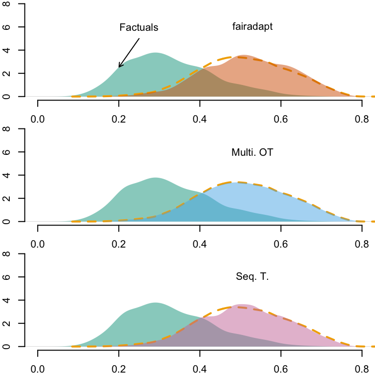
Figure 9.3: Densities of predicted scores for Black individuals with factuals and with counterfactuals. The yellow dashed line corresponds to the density of predicted scores for White individuals, using factuals.

Code

# Factuals
colours_all <- c(
  "Factual Black" = colours[["A"]],
  "Factual White" = colours[["B"]],
  "fairadapt" = colour_fpt,
  "OT" = colour_ot,
  "Seq T." = colour_seq
)

# Factuals
tb_aware_factuals <- tb_aware |> 
  filter(counterfactual == "none")
# Predicted values
pred_aware_factuals_black <- tb_aware_factuals |> filter(S == "Black") |> pull("pred")
pred_aware_factuals_white <- tb_aware_factuals |> filter(S == "White") |> pull("pred")
# Estimated densities
d_aware_factuals_black <- density(pred_aware_factuals_black)
d_aware_factuals_white <- density(pred_aware_factuals_white)

par(mfrow = c(3, 1), mar = c(2, 2, 0, 0))
x_lim <- c(0, .8)

# plot(
#   d_aware_factuals_black,
#   main = "Factuals", xlab = "", ylab = "",
#   axes = FALSE, col = NA,
#   xlim = x_lim
# )
# axis(1)
# axis(2)
# polygon(d_aware_factuals_black, col = alpha(colours[["A"]], .5), border = NA)
# polygon(d_aware_factuals_white, col = alpha(colours[["B"]], .5), border = NA)

# Fairadapt
tb_aware_fpt <- tb_aware |> 
  filter(counterfactual == "fpt")
# Predicted values, focusing on Black --> White
pred_aware_fpt_black_star <- tb_aware_fpt |> filter(S == "White") |> pull("pred")
# Estimated densities
d_aware_fpt_black_star <- density(pred_aware_fpt_black_star)

plot(
  d_aware_factuals_black,
  main = "", xlab = "", ylab = "",
  axes = FALSE, col = NA,
  xlim = x_lim
)
axis(1)
axis(2)
polygon(d_aware_factuals_black, col = alpha(colours[["A"]], .5), border = NA)
lines(d_aware_factuals_white, col = colours[["B"]], lty = 2, lwd = 2)
polygon(d_aware_fpt_black_star, col = alpha(colour_fpt, .5), border = NA)
text(x = .25, y = 6, "Factuals")
ind_min <- which.min(abs(d_aware_factuals_black$x - .2))
arrows(
  x1 = d_aware_factuals_black$x[ind_min],
  y1 = d_aware_factuals_black$y[ind_min],
  x0 = .25, 
  y0 = 5,
  length = 0.05
)
text(x = .53, y = 6, "fairadapt")

# legend(
#   ncol = 5,
#   "topleft", 
#   pch = c(19, NA, rep(19, 3)), 
#   lty = c(NA, 2, rep(NA, 3)),
#   col = colours_all,
#   legend = names(colours_all)
# )

# OT
tb_aware_ot <- tb_aware |> 
  filter(counterfactual == "ot")
# Predicted values, focusing on Black --> White
pred_aware_ot_black_star <- tb_aware_ot |> filter(S == "White") |> pull("pred")
# Estimated densities
d_aware_ot_black_star <- density(pred_aware_ot_black_star)

plot(
  d_aware_factuals_black,
  main = "", xlab = "", ylab = "",
  axes = FALSE, col = NA,
  xlim = x_lim
)
axis(1)
axis(2)
polygon(d_aware_factuals_black, col = alpha(colours[["A"]], .5), border = NA)
lines(d_aware_factuals_white, col = colours[["B"]], lty = 2, lwd = 2)
polygon(d_aware_ot_black_star, col = alpha(colour_ot, .5), border = NA)
text(x = .53, y = 6, "Multi. OT")

# Sequential transport
tb_aware_seq <- tb_aware |> 
  filter(counterfactual == "seq")
# Predicted values, focusing on Black --> White
pred_aware_seq_black_star <- tb_aware_seq |> filter(S == "White") |> pull("pred")
# Estimated densities
d_aware_seq_black_star <- density(pred_aware_seq_black_star)

plot(
  d_aware_factuals_black,
  main = "", xlab = "", ylab = "",
  axes = FALSE, col = NA,
  xlim = x_lim
)
axis(1)
axis(2)
polygon(d_aware_factuals_black, col = alpha(colours[["A"]], .5), border = NA)
lines(d_aware_factuals_white, col = colours[["B"]], lty = 2, lwd = 2)
polygon(d_aware_seq_black_star, col = alpha(colour_seq, .5), border = NA)
text(x = .53, y = 6, "Seq. T.")

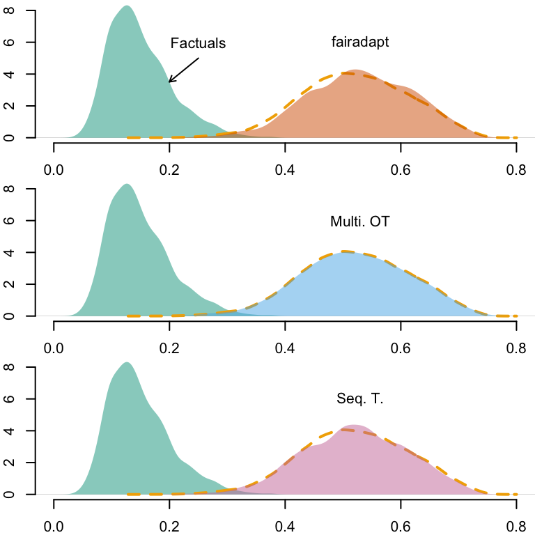
Figure 9.4: Densities of predicted scores for Black individuals with factuals and with counterfactuals. The yellow dashed line corresponds to the density of predicted scores for White individuals, using factuals.