1  Optimal Transport

Objectives

This chapter demonstrates Optimal Transport (OT) methodology applied to simulated Gaussian and general marginal distributions. The sensitive attribute \(S \in \left\{0,1\right\}\) is a binary variable, with each group \(S=0\) and \(S=1\), corresponding to a distinct Gaussian or general distribution. The objective is to transport, with OT theory, \(\boldsymbol{X} = (X_1,X_2)\) from group \(S=0\) to group \(S=1\).

# Required packages----
library(tidyverse)
library(glue)
library(igraph)
library("wesanderson")
library(scales)
library(kableExtra)
library(expm)
library(ks)

# Graphs----
colors <- c(
  `0` = "#5BBCD6", 
  `1` = "#FF0000", 
  A = "#00A08A", 
  B = "#F2AD00", 
  with = "#046C9A", 
  without = "#C93312", 
  `2` = "#0B775E"
)

# Seed
set.seed(1234)

source("../functions/utils.R")
source("../functions/graphs.R")

\(\newcommand{\indep}{\perp \!\!\! \perp}\)

1.1 Univariate Optimal Transport

1.1.1 Gaussian distribution

The Gaussian case is the most simple one since mapping \({T}^\star\), corresponding to OT, can be expressed analytically (it will be a linear mapping). Furthermore, conditional distributions of a multivariate Gaussian distribution are Gaussian distributions, and that can be used to consider an iteration of simple conditional (univariate) transports, as a substitute to joint transport \({T}^\star\). Here \(\Phi\) denotes the univariate cumulative distribution function of the standard Gaussian distribution \(\mathcal{N}(0,1)\).

One can easily prove that the optimal mapping, from a \(\mathcal{N}(\mu_0,\sigma_0^2)\) to a \(\mathcal{N}(\mu_1,\sigma_1^2)\) distribution is: \[ x_{1}={T}^\star(x_{0})= \mu_{1}+\frac{\sigma_{1}}{\sigma_{0}}(x_{0}-\mu_{0}), \] which is a nondecreasing linear transformation.

Let us illustrate this. We start by simulating two Univariate Gaussian distributions with their densities: one for the subset \(S=0\) and one for the subset \(S=1\).

# Univariate Gaussian distribution S=0
x1_grid <- seq(-5, 5, length = 251)
m0 <- -1
s0 <- 1.2
d0x1 <- dnorm(x1_grid, m0, s0)
d_0 <- data.frame(x = x1_grid, y = d0x1)

# Univariate Gaussian distribution S=1
m1 <- 1.5
s1 <- .9
d1x1 <- dnorm(x1_grid, m1, s1)
d_1 <- data.frame(x = x1_grid, y = d1x1)

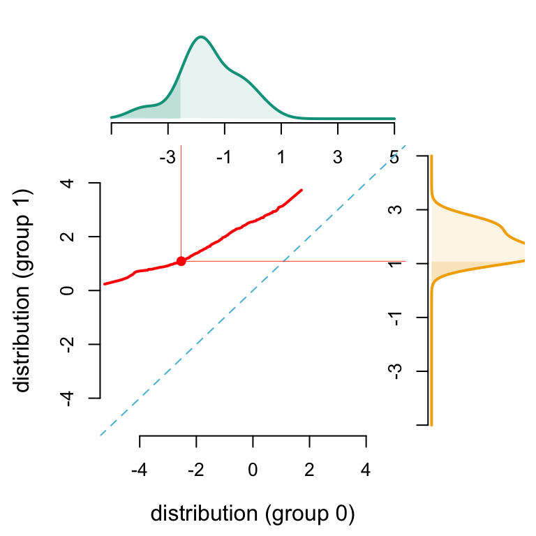
In the following graphs, we plot the optimal transport mapping for one example individual from subset \(S=0\):

u <- 0.1586553
# u-quantile of X1 for subset S=0
x1 <- qnorm(u, m0, s0)
# u-quantile of X1 for subset S=1
x1_star <- qnorm(u, m1, s1)

We also calculate the indices of \(X_1\) grid that are below this individual (\(x_1\)) and its counterfactual (\(x_1^*\)) in order to plot the cdf’s (for this individual) of \(X_1\) in both subsets \(S=0\) and \(S=1\) in the following graphs:

idx1 <- which(x1_grid <= x1)
idx1_star <- which(x1_grid <= x1_star)

We then plot the Optimal Transport line between \(X_1|S=0\) and \(X_1|S=1\):

# Graph parameters
limA <- c(-5, 5)
limB <- c(-5, 5) 
limY <- c(0, .5)
lab <- c("A", "B")
sub <- 6

{
  mat <- matrix(c(1, 2, 0, 3), 2)
  par(mfrow = c(2, 2))
  layout(mat, c(3.5, 1), c(1, 3))
  par(mar = c(0.5, 4.5, 0.5, 0.5))
}

# Density of X1 in subset S=0
plot(
  d_0$x, d_0$y, type = "l", col = colors[lab[1]], lwd = 2,
  axes = FALSE, xlab = "", ylab = "", xlim = limA, ylim = limY
)
polygon(
  c(0, d_0$x, 1), c(0, d_0$y, 0), 
  col = scales::alpha(colors[lab[1]], 0.1), 
  border = NA
)
# cdf of X1 in subset S=0
polygon(
  c(min(d_0$x), d_0$x[idx1], max(d_0$x[idx1])),
  c(0, d_0$y[idx1], 0),
  col = scales::alpha(colors["A"],.2),
  border = NA
)
# Add x-axis
axis(
  1, at = seq(limA[1], limA[2], length = sub), 
  label = c(NA, seq(limA[1], limA[2], length = sub)[-1])
)

# Optimal transport from subset S=0 to S=1 (defined with quantile functions)
par(mar = c(4.5, 4.5, 0.5, 0.5))
u_grid <- seq(0, 1, length=261)
q_0 <- qnorm(u_grid, m0, s0)
q_1 <- qnorm(u_grid, m1, s1)
plot(
  q_0, q_1, col = colors["1"], lwd = 2, type = "l", 
  xlab = "", ylab = "", xlim = limA, ylim = limB, axes = FALSE
)
abline(a = 0, b = 1, col = colors["0"], lty = 2)
# Add x-axis and y-axis
axis(1)
axis(2)
# Legend
mtext("distribution (group 0)", side = 1, line = 3, col = "black")
mtext("distribution (group 1)", side = 2, line = 3, col = "black")
# Example individual
points(x1, x1_star, pch = 19, col = colors["1"])
segments(x1, x1_star, x1, 10, lwd = .4, col = colors["1"])
segments(x1, x1_star, 10, x1_star, lwd = .4, col = colors["1"])

# Density of X1 in subset S=1
par(mar = c(4.5, 0.5, 0.5, 0.5))
plot(
  d_1$y, d_1$x, type = "l", col = colors[lab[2]], lwd = 2,
  ylim = limB, xlim = limY, xlab = "", ylab = "", axes = FALSE
)
polygon(
  c(0, d_1$y, 0), c(0, d_1$x, 1), 
  col = scales::alpha(colors[lab[2]], 0.1), border = NA
)
# cdf of X1 in subset S=1
polygon(
  c(0, d_1$y[idx1_star], 0),
  c(min(d_1$x), d_1$x[idx1_star], max(d_1$x[idx1_star])),
  col = scales::alpha(colors["B"],.2),
  border = NA
)
# Add y-axis
axis(
  2, at = seq(limB[1], limB[2], length = sub), 
  label = c(NA, seq(limB[1], limB[2], length = sub)[-c(1, sub)], NA)
)

Univariate optimal transport, with Gaussian distributions

1.1.2 General distribution

We simulate two general univariate distributions based on Gaussian distributions with their densities, cdf’s and quantile functions: one for the subset \(S=0\) and one for the subset \(S=1\).

# General distribution for subset S=0
x0 <- rnorm(13, m0, s0)
f0 <- density(x0, from = -5, to = 5, n = length(x1_grid))
d0 <- f0$y
d_0 <- data.frame(x = x1_grid, y = d0)
x0s <- sample(x0, size = 1e3, replace = TRUE) + rnorm(1e3, 0, f0$bw)
F0 <- Vectorize(function(x) mean(x0s <= x))
Q0 <- Vectorize(function(x) as.numeric(quantile(x0s, x)))

# General distribution for subset S=1
x1 <- rnorm(7, m1, 1)
f1 <- density(x1, from = -5, to = 5, n = length(x1_grid))
d1 <- f1$y
d_1 <- data.frame(x = x1_grid, y = d1)
x1s <- sample(x1, size = 1e3, replace = TRUE) + rnorm(1e3, 0, f1$bw)
F1 <- Vectorize(function(x) mean(x1s <= x))
Q1 <- Vectorize(function(x) as.numeric(quantile(x1s, x)))

In the following graphs, we plot the optimal transport mapping for one example individual from subset \(S=0\):

u <- 0.1586553
x1 <- Q0(u)
x1_star <- Q1(u)

We also calculate the indices of \(X_1\) grid that are below this individual (\(x_1\)) and its counterfactual (\(x_1^*\)) in order to plot the cdf’s (for this individual) of \(X_1\) in both subsets \(S=0\) and \(S=1\) in the following graphs:

idx1 <- which(x1_grid <= x1)
idx1_star <- which(x1_grid <= x1_star)

We then plot the Optimal Transport line between \(X_1|S=0\) and \(X_1|S=1\):

{
  mat <- matrix(c(1, 2, 0, 3), 2)
  par(mfrow = c(2, 2))
  layout(mat, c(3.5, 1), c(1, 3))
  par(mar = c(0.5, 4.5, 0.5, 0.5))
}

# Density of X1 in subset S=0
plot(d_0$x, d_0$y, type = "l", col = colors[lab[1]], lwd = 2,
     axes = FALSE, xlab = "", ylab = "", xlim = limA, ylim = limY)
polygon(c(0, d_0$x, 1), c(0, d_0$y, 0), 
        col = scales::alpha(colors[lab[1]], 0.1), 
        border = NA)
# cdf of X1 in subset S=0
polygon(
  c(min(d_0$x), d_0$x[idx1], max(d_0$x[idx1])),
  c(0, d_0$y[idx1], 0),
  col = scales::alpha(colors["A"],.2),
  border = NA
)
# Add x-axis
axis(
  1, at = seq(limA[1], limA[2], length = sub), 
  label = c(NA, seq(limA[1], limA[2], length = sub)[-1])
)

# Optimal transport from subset S=0 to S=1 (defined with quantile functions)
par(mar = c(4.5, 4.5, 0.5, 0.5))
u_grid <- seq(0, 1, length=261)
q_0 <- Q0(u_grid)
q_1 <- Q1(u_grid)
plot(
  q_0, q_1, col = colors["1"], lwd = 2, type = "l", 
  xlab = "", ylab = "", xlim = limA, ylim = limB, axes = FALSE
)
abline(a = 0, b = 1, col = colors["0"], lty = 2)
# Add x-axis and y-axis
axis(1)
axis(2)
# Legend
mtext("distribution (group 0)", side = 1, line = 3, col = "black")
mtext("distribution (group 1)", side = 2, line = 3, col = "black")
# Example individual
points(x1, x1_star, pch = 19, col = colors["1"])
segments(x1, x1_star, x1, 10, lwd = .4, col = colors["1"])
segments(x1, x1_star, 10, x1_star, lwd = .4, col = colors["1"])

# Density of X1 in subset S=1
par(mar = c(4.5, 0.5, 0.5, 0.5))
plot(
  d_1$y, d_1$x, type = "l", col = colors[lab[2]], lwd = 2,
  ylim = limB, xlim = limY, xlab = "", ylab = "", axes = FALSE
)
polygon(
  c(0, d_1$y, 0), c(0, d_1$x, 1), 
  col = scales::alpha(colors[lab[2]], 0.1), border = NA
)
# cdf of X1 in subset S=1
polygon(
  c(0, d_1$y[idx1_star], 0),
  c(min(d_1$x), d_1$x[idx1_star], max(d_1$x[idx1_star])),
  col = scales::alpha(colors["B"],.2),
  border = NA
)
# Add y-axis
axis(
  2, at = seq(limB[1], limB[2], length = sub), 
  label = c(NA, seq(limB[1], limB[2], length = sub)[-c(1, sub)], NA)
)

General marginal distribution

1.2 Multivariate Optimal Gaussian Transport

Recall that \(\boldsymbol{X}\sim\mathcal{N}(\boldsymbol{\mu},\boldsymbol{\Sigma})\) if its density, with respect to Lebesgue measure is \[ \begin{equation} {\displaystyle f(\boldsymbol{x})\propto{{\exp \left(-{\frac {1}{2}}\left({\boldsymbol{x} }-{\boldsymbol {\mu }}\right)^{\top}{\boldsymbol {\Sigma }}^{-1}\left({\boldsymbol {x} }-{\boldsymbol {\mu }}\right)\right)}.%{\sqrt {(2\pi )^{k}|{\boldsymbol {\Sigma }}|}}}} } } \end{equation} \tag{1.1}\]

If \(\boldsymbol{X}_0\sim\mathcal{N}(\boldsymbol{\mu}_0,\boldsymbol{\Sigma}_0)\) and \(\boldsymbol{X}_1\sim\mathcal{N}(\boldsymbol{\mu}_1,\boldsymbol{\Sigma}_1)\), the optimal mapping is also linear, \[ \boldsymbol{x}_{1} = T^\star(\boldsymbol{x}_{0})=\boldsymbol{\mu}_{1} + \boldsymbol{A}(\boldsymbol{x}_{0}-\boldsymbol{\mu}_{0}), \] where \(\boldsymbol{A}\) is a symmetric positive matrix that satisfies \(\boldsymbol{A}\boldsymbol{\Sigma}_{0}\boldsymbol{A}=\boldsymbol{\Sigma}_{1}\), which has a unique solution given by \(\boldsymbol{A}=\boldsymbol{\Sigma}_{0}^{-1/2}\big(\boldsymbol{\Sigma}_{0}^{1/2}\boldsymbol{\Sigma}_{1}\boldsymbol{\Sigma}_{0}^{1/2}\big)^{1/2}\boldsymbol{\Sigma}_{0}^{-1/2}\), where \(\boldsymbol{M}^{1/2}\) is the square root of the square (symmetric) positive matrix \(\boldsymbol{M}\) based on the Schur decomposition (\(\boldsymbol{M}^{1/2}\) is a positive symmetric matrix), as described in Higham (2008). If \(\boldsymbol{\Sigma}=\displaystyle\begin{pmatrix}1&r\\r&1\end{pmatrix}\), and if \(a=\sqrt{(1-\sqrt{1-r^2})/2}\), then: \[ \boldsymbol{\Sigma}^{1/2}=\displaystyle\begin{pmatrix}\sqrt{1-a^2}&a\\a&\sqrt{1-a^2}\end{pmatrix}. \]

Observe further this mapping is the gradient of the convex function \[ \psi(\boldsymbol{x})=\frac{1}{2}(\boldsymbol{x}-\boldsymbol{\mu}_0)^\top\boldsymbol{A}(\boldsymbol{x}-\boldsymbol{\mu}_0)+\boldsymbol{x}-\boldsymbol{\mu}_1^\top\boldsymbol{x} \] and \(\nabla T^\star = \boldsymbol{A}\) (see Takatsu (2011) for more properties of Gaussian transport). And if \(\boldsymbol{\mu}_0=\boldsymbol{\mu}_1=\boldsymbol{0}\), and if \(\boldsymbol{\Sigma}_{0}=\mathbb{I}\) and \(\boldsymbol{\Sigma}_{1}=\boldsymbol{\Sigma}\), \(\boldsymbol{x}_{1} = T^\star(\boldsymbol{x}_{0})=\boldsymbol{\Sigma}^{1/2}\boldsymbol{x}_{0}\). Hence, \(\boldsymbol{\Sigma}^{1/2}\) is a linear operator that maps from \(\boldsymbol{X}_0\sim\mathcal{N}(\boldsymbol{0},\mathbb{I})\) (the reference density) to \(\boldsymbol{X}_1\sim\mathcal{N}(\boldsymbol{0},\boldsymbol{\Sigma})\) (the target density).

1.3 Conditional Gaussian Transport

Alternatively, since \(\boldsymbol{\Sigma}\) is a positive definite matrix, from the Cholesky decomposition, it can be written as the product of a lower (or upper) triangular matrix and its conjugate transpose, \[ \boldsymbol{\Sigma}=\boldsymbol{L}\boldsymbol{L}^\top=\boldsymbol{U}^\top\boldsymbol{U}. \]

1.3.1 Remark

If \(\boldsymbol{\Sigma}=\displaystyle\begin{pmatrix}1&r\\r&1\end{pmatrix}\), then \(\boldsymbol{L}=\boldsymbol{\Sigma}_{2|1}^{1/2}=\displaystyle\begin{pmatrix}1&0\\r&\sqrt{1-r^2}\end{pmatrix}\) while \(\boldsymbol{U}=\boldsymbol{\Sigma}_{1|2}^{1/2}=\boldsymbol{\Sigma}_{2|1}^{1/2\top}=\boldsymbol{L}^\top\). Then \(\boldsymbol{L}^\top\boldsymbol{L}=\boldsymbol{\Sigma}=\boldsymbol{U}^\top\boldsymbol{U}\).

Both \(\boldsymbol{L}\) and \(\boldsymbol{U}\) are linear operators that map from \(\boldsymbol{X}_0\sim\mathcal{N}(\boldsymbol{0},\mathbb{I})\) (the reference density) to \(\boldsymbol{X}_1\sim\mathcal{N}(\boldsymbol{0},\boldsymbol{\Sigma})\) (the target density). \(\boldsymbol{x}_0\mapsto\boldsymbol{L}\boldsymbol{x}_0\) and \(\boldsymbol{x}_0\mapsto\boldsymbol{U}\boldsymbol{x}_0\) are respectively linear lower and upper triangular transport maps.

More generally, in dimension 2, consider the following (lower triangular) mapping \(T(x_0,y_0) = (T_x(x_0),T_{y|x}(y_0|x_0))\), \[\begin{eqnarray*} && \mathcal{N}\left( \begin{pmatrix} \mu_{0x}\\ \mu_{0y}\\ \end{pmatrix}, \begin{pmatrix} \sigma_{0x}^2 & r_0\sigma_{0x}\sigma_{0y}\\ r_0\sigma_{0x}\sigma_{0y} & \sigma_{0y}^2\\ \end{pmatrix} \right) %\\ \overset{T}{\longrightarrow} \mathcal{N}\left( \begin{pmatrix} \mu_{1x}\\ \mu_{1y}\\ \end{pmatrix}, \begin{pmatrix} \sigma_{1x}^2 & r_1\sigma_{1x}\sigma_{1y}\\ r_1\sigma_{1x}\sigma_{1y} & \sigma_{1y}^2\\ \end{pmatrix} \right), \end{eqnarray*}\]

where \(T_x(x_0)\) and \(T_{y|x}(y_0)\) are respectively \[ \begin{cases} \mu_{1x} +\displaystyle\frac{\sigma_{1x}}{\sigma_{0x}}(x_0-\mu_{0x})\phantom{\displaystyle\int}\\ \mu_{1y}+\displaystyle\frac{r_1\sigma_{1y}}{\sigma_{1x}}(T_x(x_0)-\mu_{1x})+\sqrt{\displaystyle\frac{\sigma_{0x}^2(\sigma_{1y}^2{\sigma_{1x}^2}-{r_1^2\sigma_{1y}^2})}{(\sigma_{0y}^2{\sigma_{0x}^2}-{r_0^2\sigma_{0y}^2})\sigma_{1x}^2}}(y_0\!-\!\mu_{0y}\!-\!\displaystyle\frac{r_0\sigma_{0y}}{\sigma_{0x}}(x_0\!-\!\mu_{0x})) \end{cases} \]

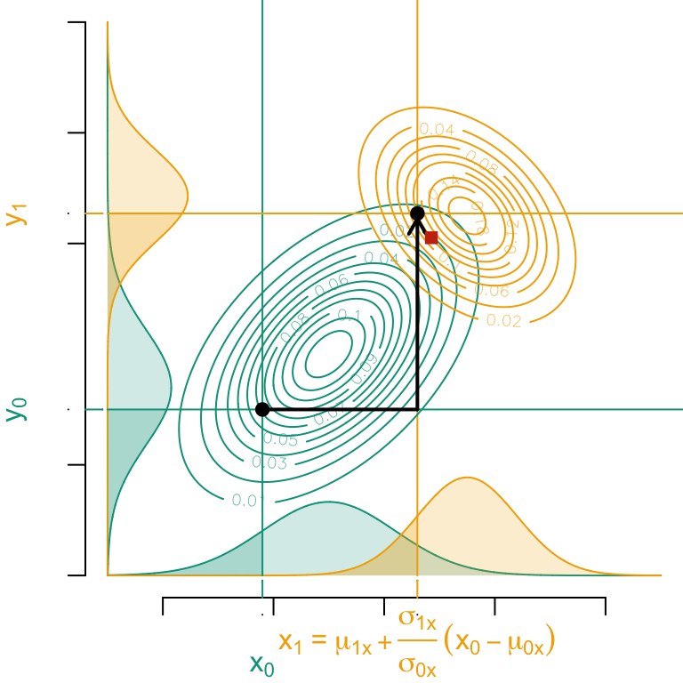
that are both linear mappings. Let us visualize this.

par(mar = c(2.5, 2.5, 0, 0))
par(mfrow = c(1, 1))

# Assumed cdf for the individual of interest
p1 <- 0.1586553
# y coordinate for that individual
b1 <- 3

vx <- seq(-5, 5, length = 6001)
vy1 <- dnorm(vx,-1, 1.2)*4
vy2 <- dnorm(vx, 1.5, .9)*4

# Marginal density of x0 in source group (at the bottom of graph)
plot(
  vx, vy1, 
  col = colors["A"], xlab = "", ylab = "", axes = FALSE, type = "l", 
  ylim = c(0, 10)
)
polygon(
  c(min(vx), vx, max(vx)),
  c(0, vy1, 0),
  col = scales::alpha(colors["A"], .2),
  border = NA
)
# Marginal density of x1 in target group (at the bottom of graph)
lines(vx, vy2, col = colors["B"])
polygon(
  c(min(vx), vx, max(vx)),
  c(0, vy2, 0),
  col = scales::alpha(colors["B"], .2),
  border = NA
)

# Corresponding quantile in the marginal distribution
a1 <- qnorm(p1, -1, 1.2) # in source group
# Transported value along x
a2 <- qnorm(p1, 1.5, .9) # in target group
# Identify observation in x below this quantile a1
idx1 <- which(vx <= a1)
# Identify observation in x below this quantile a2
idx2 <- which(vx <= a2)
# Showing P(X_1 < a1 | S = 0) on the marginal density plots
polygon(
  c(min(vx), vx[idx1], max(vx[idx1])),
  c(0, vy1[idx1],0),
  col = scales::alpha(colors["A"],.2),
  border = NA
)
# vertical line to show quantile a1
segments(a1, 0, a1, 100, col = colors["A"])
# Showing P(X_1 < a2 | S = 1) on the marginal density plots
polygon(
  c(min(vx), vx[idx2], max(vx[idx2])),
  c(0, vy2[idx2], 0),
  col=scales::alpha(colors["B"], .2),
  border = NA
)
# vertical line to show quantile a2
segments(a2, 0, a2, 100, col = colors["B"])

# Mean and variance matrix in both groups
M1 <- c(-1,-1+5)
M2 <- c(1.5,1.5+5)
S1 <- matrix(c(1,.5,.5,1)*1.2^2,2,2)
S2 <- matrix(c(1,-.4,-.4,1)*.9^2,2,2)

A <- sqrtm(S1) %*% S2 %*% (sqrtm(S1))
A <- solve(sqrtm(S1)) %*% sqrtm(A) %*% solve((sqrtm(S1)))
T <- function(x) as.vector(M2 + A %*% (x - M1))

# Bivariate Gaussian density
library(mvtnorm)
vx0 <- seq(-5, 5, length = 251)
data.grid <- expand.grid(x = vx0, y = vx0 + 5)
dgauss1 <- matrix(
  mvtnorm::dmvnorm(data.grid, mean = M1, sigma = S1), length(vx0), length(vx0)
)
dgauss2 <- matrix(
  mvtnorm::dmvnorm(data.grid, mean = M2, sigma = S2), length(vx0), length(vx0)
)

# Contour of the bivariate Gaussian density in source group
contour(vx0, vx0 + 5, dgauss1, col = colors["A"], add = TRUE)
# Contour of the bivariate Gaussian density in target group
contour(vx0, vx0 + 5, dgauss2, col = colors["B"], add = TRUE)

axis(1, at = seq(-2, 2) * 2, labels = NA)
axis(
  1, at = a1,
  labels = expression(x[0]),
  col.ticks = NA,
  col.axis = colors["A"], line = .5
)
axis(
  1, at = a2,
  labels = bquote(
    x[1]~"="~mu[1][x] + frac(sigma[1][x],sigma[0][x])~(x[0]-mu[0][x])
  ),
  col.ticks = NA,
  col.axis = colors["B"], line = .5
)
axis(
  1, at = a1,
  labels = NA,
  col.ticks = colors["A"], line = -.5
)
axis(
  1, at = a2,
  labels = NA,
  col.ticks = colors["B"], line = -.5
)

###
# Second axis
###
y <- b1
vx <- vx + 5
mu1 <- M1[2] + S1[1, 2] / S1[1, 1] * (a1 - M1[1])
sig1 <- sqrt(S1[2, 2] - S1[2, 1]^2 / S1[2, 2])
mu2 <- M2[2] + S2[1, 2] / S2[1, 1] * (a2 - M2[1])
sig2 <- sqrt(S2[2, 2]- S2[2, 1]^2 / S2[2, 2])
vz1 <- dnorm(vx, mu1, sig1) * 3
vz2 <- dnorm(vx, mu2, sig2) * 3

# Marginal density on y, source group
lines(vz1 - 5, vx, col = colors["A"])
polygon(
  c(0, vz1, 0) - 5,
  c(min(vx), vx, max(vx)),
  col = scales::alpha(colors["A"], .2),
  border = NA
)
# target group
lines(vz2 - 5, vx, col = colors["B"])
polygon(
  c(0, vz2, 0) - 5,
  c(min(vx), vx, max(vx)),
  col = scales::alpha(colors["B"], .2),
  border = NA
)

# Identify the cdf at b1 in the marginal distribution
p1 <- pnorm(b1, mu1, sig1)
# Transported value in the target marginal distribution
b2 <- qnorm(p1, mu2, sig2)
# Identify observation in y below this quantile b1
idx1 <- which(vx <= b1)
# Identify observation in y below this quantile b2
idx2 <- which(vx <= b2)
# Showing P(X_2 < b1 | S = 0) on the marginal density plots
polygon(
  c(0, vz1[idx1], 0) - 5,
  c(min(vx), vx[idx1], max(vx[idx1])),
  col = scales::alpha(colors["A"], .2),
  border = NA
)
# Showing P(X_2 < b2 | S = 1) on the marginal density plots
polygon(
  c(0, vz2[idx2], 0) - 5,
  c(min(vx), vx[idx2], max(vx[idx2])),
  col = scales::alpha(colors["B"], .2),
  border = NA
)
# horizontal line to show quantile b1
segments(-5, b1, 100, b1, col = colors["A"])
# horizontal line to show quantile b2
segments(-5, b2, 100, b2, col = colors["B"])

# Draw the individual of interest 
points(a1, b1, pch = 19)


axis(2, at = c(0,1,3,4,5) * 2, labels = NA)
axis(
  2, at = b1,
  labels = expression(y[0]),
  col.ticks = NA,
  col.axis = colors["A"], line = .5
)
axis(
  2, at = b2,
  labels = bquote(y[1]),
  col.ticks = NA,
  col.axis = colors["B"], line = .5
)
axis(
  2,at = b1,
  labels = NA,
  col.ticks = colors["A"], line = -.5
)
axis(
  2,at = b2,
  labels = NA,
  col.ticks = colors["B"], line = -.5
)

# Drawing transported point
points(a2, b2, pch = 19)

# Decomposition of the sequential transport
# First transport along the x axis
segments(a1, b1, a2, b1, lwd = 2)
# Then transport along the y axis
arrows(a2, b1, a2, b2 - .1, length = .1, lwd = 2)

# Storing in a matrix the coordinates of the point before and after transport
X_then_Y <- matrix(c(a1, b1, a2, b2), 2, 2)
colnames(X_then_Y) = c("start","x_then_y")

# Showing the transported point if we assume another sequential transport:
# first along the y axis, and then along the x axis
M1 <- c(-1, -1+5)
M2 <- c(1.5, 1.5)
S1 <- matrix(c(1, .5, .5, 1) * 1.2^2, 2, 2)
S2 <- matrix(c(1, -.4, -.4, 1) * .9^2, 2, 2)

# Transport
AA <- sqrtm(S1) %*% S2 %*% (sqrtm(S1))
AA <- solve(sqrtm(S1)) %*% sqrtm(AA) %*% solve((sqrtm(S1)))
T <- function(x) as.vector(M2 + AA %*% (x - M1))
opt_transp <- T(c(a1, b1))
XYopt <- matrix(c(a1, b1, opt_transp[1], opt_transp[2] + 5), 2, 2)
colnames(XYopt) = c("start","OT")

# Drawing the point transported with the different order in the sequence
points(opt_transp[1], opt_transp[2] + 5, pch = 15, col = "#C93312")

Gaussian conditional optimal transport. The process begins with a univariate transport along the \(x\) axis (using \(T_x^*\)), followed by a transport along the \(y\) axis on the conditional distribution (using \(T_{y|x}^*\)), corresponding to the “lower triangular affine mapping.” The red square is the multivariate optimal transport of the point considering an “upper triangular affine mapping” instead.

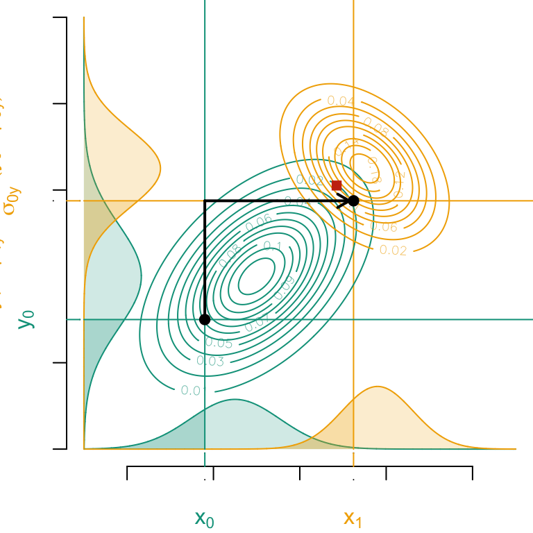
Now, let us transport first along the \(y\) axis, and then along the \(x\) axis.

par(mar = c(2.5, 2.5, 0, 0))
par(mfrow = c(1, 1))

# Mean and variance matrix in both groups
M1 <- c(-1, -1 + 5)
M2 <- c(1.5, 1.5 + 5)
S1 <- matrix(c(1,.5,.5,1)*1.2^2,2,2)
S2 <- matrix(c(1,-.4,-.4,1)*.9^2,2,2)

# Quantile for the observartion of interest, in the distribution of x
a1 <- -2.2
# y coordinate for the individual of interest
b1 <- 3
b2 <- qnorm(pnorm(b1, 5 - 1, 1.2), 5 + 1.5, .9)

mu1 <- M1[2] + S1[1, 2] / S1[1, 1] * (b1 - M1[1] - 5)
sig1 <- sqrt(S1[2, 2] - S1[2, 1]^2 / S1[2, 2])
mu2 <- M2[2] + S2[1, 2] / S2[1, 1] * (b2 - M2[1] - 5)
sig2 <- sqrt(S2[2, 2] - S2[2, 1]^2 / S2[2, 2])

# Assumed cdf for the individual of interest
p1 <- pnorm(a1 + 5, mu1, sig1)

vx <- seq(-5, 5, length = 6001)
vx <- vx+5
vy1 <- dnorm(vx, mu1, sig1) * 3
vy2 <- dnorm(vx, mu2, sig2) * 3

vz1 <- dnorm(vx - 5, -1, 1.2) * 4
vz2 <- dnorm(vx - 5, 1.5, .9) * 4

# Marginal density of x0 in source group (at the bottom of graph)
plot(
  vx, vy1,
  col = colors["A"], xlab = "", ylab = "", axes = FALSE, 
  type = "l", ylim = c(0, 10)
)
lines(vz1 - 5, vx, col = colors["A"])
polygon(
  c(min(vx), vx, max(vx)),
  c(0, vy1, 0),
  col = scales::alpha(colors["A"], .2),
  border = NA
)
# Marginal density of x1 in target group (at the bottom of graph)
lines(vx, vy2, col = colors["B"])
polygon(
  c(min(vx), vx, max(vx)),
  c(0, vy2, 0),
  col = scales::alpha(colors["B"], .2),
  border = NA
)


# Transported value along x
a2 <- qnorm(p1, mu2, sig2)
a1 <- a1 + 5
# Identify observation in x below this quantile a1
idx1 <- which(vx <= a1)
# Identify observation in x below this quantile a2
idx2 <- which(vx <= a2)
# Showing P(X_1 < a1 | S = 0) on the marginal density plots
polygon(
  c(min(vx), vx[idx1], max(vx[idx1])),
  c(0, vy1[idx1], 0),
  col = scales::alpha(colors["A"], .2),
  border = NA
)
# vertical line to show quantile a1
segments(a1, 0, a1, 100, col = colors["A"])
# Showing P(X_1 < a2 | S = 1) on the marginal density plots
polygon(
  c(min(vx), vx[idx2], max(vx[idx2])),
  c(0, vy2[idx2], 0),
  col = scales::alpha(colors["B"], .2),
  border = NA
)
# vertical line to show quantile a2
segments(a2, 0, a2, 100, col = colors["B"])

# Bivariate Gaussian density
library(mvtnorm)
vx0 <- seq(-5, 5, length = 251)
data.grid <- expand.grid(x = vx0, y = vx0 + 5)
dgauss1 <- matrix(
  mvtnorm::dmvnorm(data.grid, mean = M1, sigma = S1), length(vx0), length(vx0)
)
dgauss2 <- matrix(
  mvtnorm::dmvnorm(data.grid, mean = M2, sigma = S2), length(vx0), length(vx0)
)

# Contour of the bivariate Gaussian density in source group
contour(vx0 + 5,vx0 + 5, dgauss1, col = colors["A"], add = TRUE)
# Contour of the bivariate Gaussian density in target group
contour(vx0 + 5, vx0 + 5, dgauss2, col = colors["B"], add = TRUE)


# Showing and annoting x axis
axis(1, at = 5 + seq(-2, 2) * 2, labels = NA)
axis(
  1, at = a1,
  labels = expression(x[0]),
  col.ticks = NA,
  col.axis = colors["A"], line = .5
)
axis(
  1, at = a2,
  labels = bquote(x[1]),
  col.ticks = NA,
  col.axis = colors["B"], line = .5
)
axis(
  1, at = a1,
  labels = NA,
  col.ticks = colors["A"], line = -.5
)
axis(
  1, at = a2,
  labels = NA,
  col.ticks = colors["B"], line = -.5
)

###
# Second axis
###

# Marginal density on y, source group
lines(vz1, vx, col = colors["A"])
polygon(
  c(0, vz1, 0),
  c(min(vx), vx, max(vx)),
  col = scales::alpha(colors["A"], .2),
  border = NA
)
# target group
lines(vz2, vx, col = colors["B"])
polygon(
  c(0, vz2, 0),
  c(min(vx), vx, max(vx)),
  col = scales::alpha(colors["B"], .2),
  border = NA
)

# Identify the cdf at b1 in the marginal distribution
p1 <- pnorm(b1, 5 - 1, 1.2)
# Transported value in the target marginal distribution
b2 <- qnorm(p1, 5 + 1.5, .9)
# Identify observation in y below this quantile b1
idx1 <- which(vx <= b1)
# Identify observation in y below this quantile b2
idx2 <- which(vx <= b2)
# Showing P(X_2 < b1 | S = 0) on the marginal density plots
polygon(
  c(0, vz1[idx1], 0),
  c(min(vx), vx[idx1], max(vx[idx1])),
  col = scales::alpha(colors["A"], .2),
  border = NA
)
# Showing P(X_2 < b2 | S = 1) on the marginal density plots
polygon(
  c(0, vz2[idx2], 0),
  c(min(vx), vx[idx2], max(vx[idx2])),
  col = scales::alpha(colors["B"], .2),
  border = NA
)

# horizontal line to show quantile b1
segments(0, b1, 100, b1, col = colors["A"])
# horizontal line to show quantile b2
segments(0, b2, 100, b2, col = colors["B"])

# Draw the individual of interest 
points(a1, b1, pch = 19)

# Drawing y axis
axis(2, at = c(0, 1, 3, 4, 5) * 2, labels = NA)
axis(
  2, at = b1,
  labels = expression(y[0]),
  col.ticks = NA,
  col.axis = colors["A"], line = 0
)
axis(
  2, at = b2,
  labels = bquote(
    y[1]~"="~mu[1][y]+frac(sigma[1][y],sigma[0][y])~(y[0]-mu[0][y])
  ),
  col.ticks = NA,
  col.axis = colors["B"], line = .5
)
axis(
  2, at = b1,
  labels=NA,
  col.ticks = colors["A"],line = -.5
)
axis(
  2,at = b2,
  labels = NA,
  col.ticks = colors["B"], line = -.5
)

# Drawing transported point
points(a2, b2, pch = 19)

# Decomposition of the sequential transport
# First transport along the x axis
segments(a1, b1, a1, b2, lwd = 2)
# Then transport along the y axis
arrows(a1, b2, a2 - .1, b2, length = .1, lwd = 2)

# Storing in a matrix the coordinates of the point before and after transport
Y_then_X = matrix(c(a1, b1, a2, b2), 2, 2)
colnames(Y_then_X) = c("start","y_then_x")

# Showing the transported point if we assume another sequential transport:
# first along the x axis, and then along the y axis
M1 <- c(-1, -1)
M2 <- c(1.5, 1.5)
S1 <- matrix(c(1, .5, .5, 1) * 1.2^2, 2, 2)
S2 <- matrix(c(1, -.4, -.4, 1) * .9^2, 2, 2)

# Transport
AA <- sqrtm(S1) %*% S2 %*% (sqrtm(S1))
AA <- solve(sqrtm(S1)) %*% sqrtm(AA) %*% solve((sqrtm(S1)))
T <- function(x) as.vector(M2 + AA %*% (x - M1))
opt_transp <- T(c(a1 - 5, b1 - 5))

# Drawing the point transported with the different order in the sequence
points(opt_transp[1] + 5, opt_transp[2] + 5, pch = 15, col = "#C93312")

Gaussian conditional optimal transport. The process begins with a univariate transport along the \(y\) axis (using \(T_y^*\)), followed by a transport along the \(x\) axis on the conditional distribution (using \(T_{x|y}^*\)), corresponding to the “upper triangular affine mapping.” The red square is the multivariate optimal transport of the point considering a “lower triangular affine mapping” instead.

Of course, this is highly dependent on the axis parametrization. Instead of considering projections on the axis, one could consider transport in the direction \(\overrightarrow{u}\), followed by transport in the direction \(\overrightarrow{u}^\perp\) (on conditional distributions). This will be visualized in Figure 1.1 and Figure 1.2

1.4 Gaussian Probabilistic Graphical Models

An interesting feature of the Gaussian multivariate distribution is that any marginal and any conditional distribution (given other components) is still Gaussian. More precisely, if \[ {\displaystyle \boldsymbol {x} ={\begin{pmatrix}\boldsymbol {x} _{1}\\\boldsymbol {x} _{2}\end{pmatrix}}},~{\displaystyle {\boldsymbol {\mu }}={\begin{pmatrix}{\boldsymbol {\mu }}_{1}\\{\boldsymbol {\mu }}_{2}\end{pmatrix}}}\text{ and } {\displaystyle {\boldsymbol {\Sigma }}={\begin{pmatrix}{\boldsymbol {\Sigma }}_{11}&{\boldsymbol {\Sigma }}_{12}\\{\boldsymbol {\Sigma }}_{21}&{\boldsymbol {\Sigma }}_{22}\end{pmatrix}}}, \] then \(\boldsymbol{X}_1\sim\mathcal{N}(\boldsymbol{\mu}_1,\boldsymbol{\Sigma}_{11})\), while, with notations of Equation 1.1, we can also write \({\displaystyle { {\boldsymbol {B }_{1}}}={\boldsymbol {B }}_{11}-{\boldsymbol {B }}_{12}{\boldsymbol {B }}_{22}^{-1}{\boldsymbol {B }}_{21}}\) (based on properties of inverses of block matrices, also called the Schur complement of a block matrix). Furthermore, conditional distributions are also Gaussian, \(\boldsymbol{X}_1|\boldsymbol{X}_2=\boldsymbol{x}_2\sim\mathcal{N}({\boldsymbol {\mu }_{1|2}},{\boldsymbol {\Sigma }_{1|2}}),\) \[ \begin{cases} {\displaystyle { {\boldsymbol {\mu }_{1|2}}}={\boldsymbol {\mu }}_{1}+{\boldsymbol {\Sigma }}_{12}{\boldsymbol {\Sigma }}_{22}^{-1}\left(\boldsymbol{x}_2 -{\boldsymbol {\mu }}_{2}\right)} \\ {\displaystyle { {\boldsymbol {\Sigma }_{1|2}}}={\boldsymbol {\Sigma }}_{11}-{\boldsymbol {\Sigma }}_{12}{\boldsymbol {\Sigma }}_{22}^{-1}{\boldsymbol {\Sigma }}_{21},} \end{cases} \] and the inverse of the conditional variance is simply \(\boldsymbol {B }_{11}\).

It is well known that if \(\boldsymbol{X}\sim\mathcal{N}(\boldsymbol{\mu},\boldsymbol{\Sigma})\), \(X_i\indep X_j\) if and only if \(\Sigma_{i,j}=0\). More interestingly, we also have the following result, initiated by :

Proposition

If \(\boldsymbol{X}\sim\mathcal{N}(\boldsymbol{\mu},\boldsymbol{\Sigma})\), with notations of Equation 1.1, \(\boldsymbol{B}=\boldsymbol{\Sigma}^{-1}\), \(\boldsymbol{X}\) is Markov with respect to \(\mathcal{G}=(E,V)\) if and only if \(B_{i,j}=0\) whenever \((i,j),(j,i)\notin E\).

Proof

This is a direct consequence of the following property : if \(\boldsymbol{X}\sim\mathcal{N}(\boldsymbol{\mu},\boldsymbol{\Sigma})\), \(X_i\indep X_j |\boldsymbol{X}_{-i,j}\) if and only if \(B_{i,j}=0\) (since the log-density has separate terms in \(x_i\) and \(x_j\)).

1.5 Sequential transport

In the Gaussian case we obviously recover the results of Section 1.3, if we plug Gaussian distributions in the expressions shown in the “Sequential Transport” of the paper: \[ \begin{cases} X_{0:1}\!\sim\!\mathcal{N}(\mu_{0:1},\sigma_{0:1}^2),\text{ hence }F_{0:1}(x)\!=\!\Phi\big(\sigma_{0:1}^{-1}(x\!-\!\mu_{0:1})\big)\\ X_{1:1}\!\sim\!\mathcal{N}(\mu_{1:1},\sigma_{1:1}^2),\text{ hence }F_{1:1}^{-1}(u)\!=\!\mu_{1:1}\!+\!\sigma_{1:1}\!\Phi^{-1}(u) \end{cases} \] thus \[ T_1^\star(x) = F_{1:1}^{-1}\big(F_{0:1}(x)\big)=\mu_{1:1} +\displaystyle\frac{\sigma_{1:1}}{\sigma_{0:1}}(x-\mu_{0:1}), \] while \[ \begin{cases} X_{0:2}|x_{0:1}\sim\mathcal{N}(\mu_{0:2|1},\sigma_{0:2|1}^2),\\ X_{1:2}|x_{0:1}\sim\mathcal{N}(\mu_{1:2|1},\sigma_{1:2|1}^2),\\ \end{cases} \] i.e., \[ \begin{cases} F_{0:2|1}(x)=\Phi\big(\sigma_{0:2|1}^{-1}(x-\mu_{0:2|1})\big),\\ F_{1:2|1}^{-1}(u)=\mu_{1:2|1}+\sigma_{1:2|1}\Phi^{-1}(u), \end{cases} \] where we consider \(X_{0:2}\) conditional to \(X_{0:1}=x_{0:1}\) in the first place, \[ \begin{cases} \mu_{0:2|1} = \mu_{0:2} +\displaystyle\frac{\sigma_{0:2}}{\sigma_{0:1}}(x_{0:1}-\mu_{0:1}),\phantom{\displaystyle\int}\\ \sigma_{0:2|1}^2 = \sigma_{0:2}^2 -\displaystyle\frac{r^2_0\sigma_{0:2}^2}{\sigma_{0:1}^2},\phantom{\int} \end{cases} \] and \(X_{1:2}\) conditional to \(X_{1:1}=T^\star_1(x_{0:1})\) in the second place, \[ \begin{cases} \mu_{1:2|1} = \mu_{1:2} +\displaystyle\frac{\sigma_{1:2}}{\sigma_{1:1}}\big(T^\star_1(x_{0:1})-\mu_{1:1}\big),\phantom{\int}\\ \sigma_{1:2|1}^2= \sigma_{1:2}^2 -\displaystyle\frac{r^2_1\sigma_{1:2}^2}{\sigma_{1:1}^2},\phantom{\int} \end{cases} \] thus \[ T_{2|1}(x) = F_{1:2|1}^{-1}\big(F_{0:2|1}(x)\big)=\mu_{1:2|1} +\displaystyle\frac{\sigma_{1:2|1}}{\sigma_{0:2|1}}(x-\mu_{0:2|1}), \] which is \[ \begin{eqnarray*} &&\mu_{1:2}+\displaystyle\frac{r_1\sigma_{1:2}}{\sigma_{1:1}}\big(\mu_{1:1} +\displaystyle\frac{\sigma_{1:1}}{\sigma_{0:1}}(x_{0:1}-\mu_{0:1})-\mu_{1:1}\big) \\&&+\sqrt{\frac{\sigma_{0:1}^2(\sigma_{1:2}^2{\sigma_{1:1}^2}-{r_1^2\sigma_{1:2}^2})}{(\sigma_{0:2}^2{\sigma_{0:1}^2}-{r_0^2\sigma_{0:2}^2})\sigma_{1:1}^2}}\cdot\big(x-\mu_{0:2}-\displaystyle\frac{r_0\sigma_{0:2}}{\sigma_{0:1}}(x_{0:1}-\mu_{0:1})\big). \end{eqnarray*} \]

1.6 General Conditional Transport

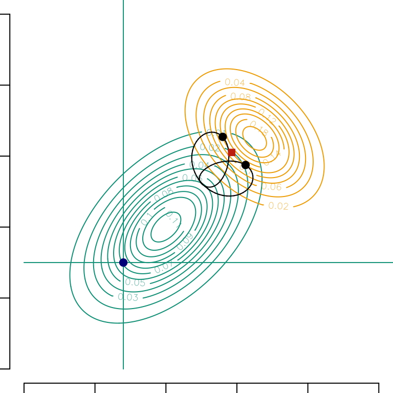
An interesting property of Gaussian vectors is the stability under rotations. In dimension 2, instead of a sequential transport of \(\boldsymbol{x}\) on \(\overrightarrow{e}_x\) and then (conditionally) on $_y, one could consider a projection on any unit vector \(\overrightarrow{u}\) (with angle \(\theta\)), and then (conditionally) along the orthogonal direction \(\displaystyle \overrightarrow{u}^\perp\). In Figure 1.1, we can visualize the set of all counterfactuals \(\boldsymbol{x}^\star\) when \(\theta\in[0,2\pi]\). The (global) optimal transport is also considered (shown with a red square).

angle <- function(theta,
                  A = c(-2.2,-2)) {
  
  # Rotation
  R <- matrix(c(cos(theta), sin(theta), -sin(theta), cos(theta)), 2, 2)
  # Mean and Variance
  M1 <- c(-1, -1)
  M2 <- c(1.5, 1.5)
  S1 <- matrix(c(1, .5, .5, 1) * 1.2^2, 2, 2)
  S2 <- matrix(c(1, -.4, -.4, 1) * .9^2, 2, 2)
  
  # After applying the rotation
  M1 <- as.vector(R %*% M1)
  M2 <- as.vector(R %*% M2)
  S1 <- t(R) %*% S1 %*% R
  S2 <- t(R) %*% S2 %*% R
  A <- as.vector(R %*% A)
  
  # Coordinates
  a1 <- A[1]
  b1 <- A[2]
  a2 <- qnorm(pnorm(a1, M1[1], sqrt(S1[1, 1])), M2[1], sqrt(S2[1, 1]))
  mu1 <- M1[2] + S1[1, 2] / S1[1, 1] * (a1 - M1[1])
  sig1 <- sqrt(S1[2, 2] - S1[2, 1]^2 / S1[2, 2])
  mu2 <- M2[2] + S2[1, 2] / S2[1, 1] * (a2 - M2[1])
  sig2 <- sqrt(S2[2, 2] - S2[2, 1]^2 / S2[2, 2])
  p1 <- pnorm(b1, mu1, sig1)
  b2 <- qnorm(p1, mu2, sig2)
  B <- c(a2, b2)
  
  c(
    as.vector(t(R) %*% A),
    as.vector(t(R) %*% B)
  )
}

# Mean and variance
M1 <- c(-1, -1)
M2 <- c(1.5, 1.5)
S1 <- matrix(c(1, .5, .5, 1) * 1.2^2, 2, 2)
S2 <- matrix(c(1, -.4, -.4, 1) * .9^2, 2, 2)

A <- c(-2.2, -2)

par(mfrow = c(1, 1), mar = c(.5, .5, 0, 0))

# Bivariate Gaussian density
library(mvtnorm)
vx0 <- seq(-5, 5, length = 251)
data.grid <- expand.grid(x = vx0, y = vx0)
dgauss1 <- matrix(
  mvtnorm::dmvnorm(data.grid, mean = M1, sigma = S1), length(vx0), length(vx0)
)
dgauss2 <- matrix(
  mvtnorm::dmvnorm(data.grid, mean = M2, sigma = S2), length(vx0), length(vx0)
)

# Contour of the bivariate Gaussian density in source group
contour(
  vx0, vx0, dgauss1, col = colors["A"], 
  xlim = c(-5, 5), ylim = c(-5, 5), axes = FALSE
)
# Contour of the bivariate Gaussian density in target group
contour(vx0, vx0, dgauss2, col = colors["B"], add = TRUE)

# Horizontal and vertical line showing the coordinates of the point of interest
segments(A[1], -5, A[1], 100, col = colors["A"])
segments(-5, A[2], 100, A[2], col = colors["A"])
# Drawing this point
points(A[1], A[2], pch = 19, col = "darkblue")

# Add axes
axis(1, at = c(0, 1, 2, 3, 4, 5) * 2 - 5, labels = NA)
axis(2, at = c(0, 1, 2, 3, 4, 5) * 2 - 5, labels = NA)

# Apply rotations
MANGLE <- Vectorize(angle)(seq(0, 2 * pi, length = 100))
# Draw the transported points for each rotation
lines(MANGLE[3, ], MANGLE[4, ])

# Display specific point when transporting first along the x axis and then the
# orthogonal axis, i.e., y
m <- angle(0, c(-2.2, -2))
points(m[3],m[4],pch=19)

# Same but transporting first along the y axis and then on the orthogonal axis,
# i.e., x
m <- angle(pi/2, c(-2.2, -2))
points(m[3], m[4], pch = 19)

# Global optimal transport
T <- function(x) as.vector(M2 + AA %*% (x - M1))
opt_transp <- T(c(A[1], A[2]))
points(opt_transp[1], opt_transp[2], pch = 15, col = "#C93312")

Figure 1.1: Gaussian conditional optimal transports. The process begins with a univariate transport along the direction \(\overrightarrow{u}\) (using \(\displaystyle T^\star_{\overrightarrow{u}}\)) followed by a transport along the orthogonal direction \(\displaystyle \overrightarrow{u}^\perp\), on conditional distributions (using \(\displaystyle T^\star_{\overrightarrow{u}^\perp|{\overrightarrow{u}}}\)). The blue point is the starting point. The curves in the upper right corner represent the set of all transport maps of the same point (bottom left corner) for all possible directions \(\displaystyle \overrightarrow{u}\), the black points correspond to classical \(x\) (horizontal) and \(y\) (vertical) directions. The red square shows the global optimal tranpport.

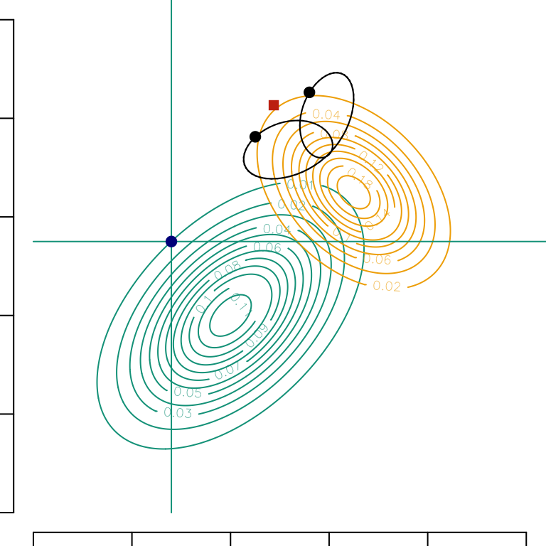
We can consider another starting point.

# Consider the following starting point
A = c(-2.2, .5)

par(mfrow = c(1, 1), mar = c(.5, .5, 0, 0))

# Bivariate Gaussian density
vx0 <- seq(-5, 5, length = 251)
data.grid <- expand.grid(x = vx0, y = vx0)
dgauss1 <- matrix(
  mvtnorm::dmvnorm(data.grid, mean = M1, sigma = S1), length(vx0), length(vx0)
)
dgauss2 <- matrix(
  mvtnorm::dmvnorm(data.grid, mean = M2, sigma = S2), length(vx0), length(vx0)
)
# Contour of the bivariate Gaussian density in source group
contour(
  vx0, vx0, dgauss1, col = colors["A"], 
  xlim = c(-5, 5), ylim = c(-5, 5), axes = FALSE
)
# Contour of the bivariate Gaussian density in target group
contour(vx0, vx0, dgauss2, col = colors["B"], add = TRUE)

# Vertical and horizontal lines showing the coordinates of the point
segments(A[1], -5, A[1], 100, col = colors["A"])
segments(-5, A[2], 100, A[2], col = colors["A"])
# Drawing that starting point
points(A[1], A[2], pch = 19, col = "darkblue")

# Showing axes
axis(1, at = c(0,1,2,3,4,5) * 2 - 5, labels = NA)
axis(2, at = c(0,1,2,3,4,5) * 2 - 5, labels = NA)

# Apply rotations
MANGLE <- 
  Vectorize(function(x) angle(x, c(-2.2, .5)))(seq(0, 2 * pi, length = 100))
# Draw the transported points for each rotation
lines(MANGLE[3, ], MANGLE[4, ])

# Display specific point when transporting first along the x axis and then the
# orthogonal axis, i.e., y
m <- angle(0, c(-2.2, .5))
points(m[3], m[4], pch = 19)

# Same but transporting first along the y axis and then on the orthogonal axis,
# i.e., x
m <- angle(pi/2, c(-2.2, .5))
points(m[3], m[4], pch = 19)

# Global optimal transport
AA <- sqrtm(S1) %*% S2 %*% (sqrtm(S1))
AA <- solve(sqrtm(S1)) %*% sqrtm(AA) %*% solve((sqrtm(S1)))
T <- function(x) as.vector(M2 + AA %*% (x - M1))
opt_transp <- T(c(A[1], A[2]))
points(opt_transp[1], opt_transp[2], pch = 15, col = "#C93312")

Figure 1.2: Gaussian conditional optimal transports. The process begins with a univariate transport along the direction \(\overrightarrow{u}\) (using \(\displaystyle T^\star_{\overrightarrow{u}}\)) followed by a transport along the orthogonal direction \(\displaystyle \overrightarrow{u}^\perp\), on conditional distributions (using \(\displaystyle T^\star_{\overrightarrow{u}^\perp|{\overrightarrow{u}}}\)). The blue point is the starting point. The curves in the upper right corner represent the set of all transport maps of the same point (bottom left corner) for all possible directions \(\displaystyle \overrightarrow{u}\), the black points correspond to classical \(x\) (horizontal) and \(y\) (vertical) directions. The red square shows the global optimal tranpport.

Higham, Nicholas J. 2008. Functions of Matrices: Theory and Computation. SIAM.

Takatsu, Asuka. 2011. “Wasserstein Geometry of Gaussian Measures.” Osaka Journal of Mathematics 48 (4): 1005–26.