This chapter adopts a naive approach to construct counterfactuals \(\boldsymbol{x}^\star\) : the sensitive attribute is simply set to \(s \leftarrow 1\) , while all other characteristics remain unchanged (the ceteris paribus approach). The aware and unaware classifiers \(m(\cdot)\) (see Chapter 7 ) are then applied to make new predictions \(m(s=1,\boldsymbol{x}^\star)\) for individuals in the protected class, i.e., observations in \(\mathcal{D}_0\) .
In the article, we use four methods to create counterfactuals:
Naive approach (this chapter)
Fairadapt (Chapter 9 )
Multivariate optimal transport (Chapter 10 )
Sequential transport (the methodology we develop in the paper, see Chapter 11 ).
Required packages and definition of colours.
# Required packages---- library (tidyverse)library (fairadapt)library (devtools)load_all ("../seqtransfairness/" )# Graphs---- = font_title = 'Times New Roman' :: loadfonts (quiet = T)= 'plain' = 'plain' = 14 = 11 = 11 <- function () {theme_minimal () %+replace% theme (text = element_text (family = font_main, size = size_text, face = face_text),legend.text = element_text (family = font_main, size = legend_size),axis.text = element_text (size = size_text, face = face_text), plot.title = element_text (family = font_title, size = size_title, hjust = 0.5 plot.subtitle = element_text (hjust = 0.5 )# Seed set.seed (2025 )<- c ("source" = "#00A08A" ,"reference" = "#F2AD00" ,"naive" = "gray"
Load Data and Classifier
We load the dataset where the sensitive attribute (\(S\) ) is the race, obtained Chapter 6.3 :
load ("../data/df_race.rda" )
We also load the dataset where the sensitive attribute is also the race, but where where the target variable (\(Y\) , ZFYA) is binary (1 if the student obtained a standardized first year average over the median, 0 otherwise). This dataset was saved in Chapter 7.5 :
load ("../data/df_race_c.rda" )
We also need the predictions made by the classifier (see Chapter 7 ):
# Predictions on train/test sets load ("../data/pred_aware.rda" )load ("../data/pred_unaware.rda" )# Predictions on the factuals, on the whole dataset load ("../data/pred_aware_all.rda" )load ("../data/pred_unaware_all.rda" )
Counterfactuals with the Naive Approach
We begin with the reference class being Black individuals (minority group). We set the sensitive variable (race) of Black individuals into the value of the majority group, i.e., White.
<- pred_unaware$ model<- predict (newdata = df_race_c |> select (S, X1, X2) |> filter (S == "Black" ) |> mutate (S = "White" ), type = "response" <- pred_aware$ model<- predict (newdata = df_race_c |> select (S, X1, X2) |> filter (S == "Black" ) |> mutate (S = "White" ), type = "response"
We build two tables, one for the unaware model, the other for the aware model, with the predicted values using the naive version of the counterfactuals.
<- |> filter (S == "Black" ) |> mutate (S_origin = S,S = "White" ,pred = pred_unaware_naive_black,type = "counterfactual" |> mutate (id_indiv = row_number ())<- |> filter (S == "Black" ) |> mutate (S_origin = S,S = "White" ,pred = pred_aware_naive_black,type = "counterfactual" |> mutate (id_indiv = row_number ())
Unaware Model
The predicted values using the initial characteristics (the factuals), for the unaware model are stored in the object pred_unaware_all. We put in a table the initial characteristics (factuals) and the prediction made by the unaware model:
<- tibble (S = df_race_c$ S,S_origin = df_race_c$ S,X1 = df_race_c$ X1,X2 = df_race_c$ X2,Y = df_race_c$ Y,pred = pred_unaware_all,type = "factual" |> mutate (id_indiv = row_number ())
<- |> mutate (S_origin = S) |> bind_rows (counterfactuals_unaware_naive_black)
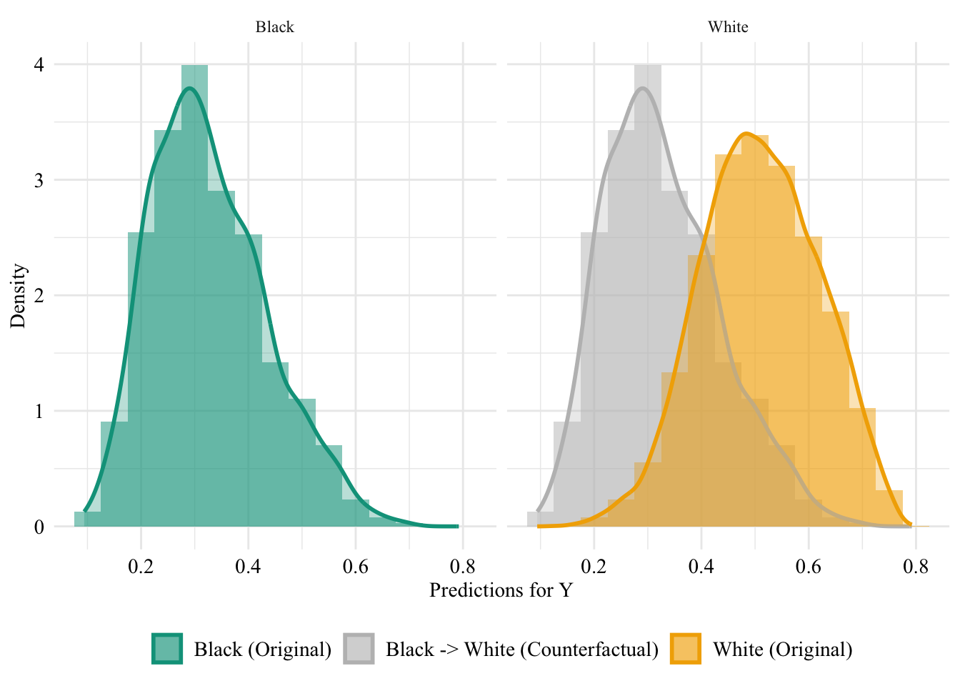
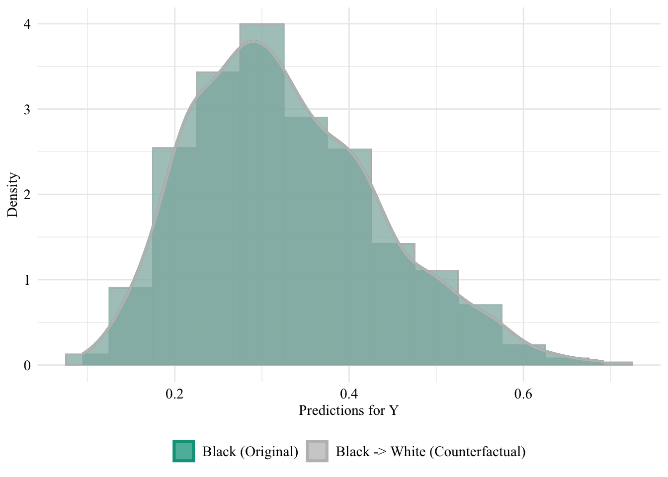
The unaware model is blind to the sensitive attribute. Hence, changing the sensitive attribute does not affect the predicted scores.
Codes used to create the Figure.
ggplot (|> mutate (group = case_when (== "Black" & S == "Black" ~ "Black (Original)" ,== "Black" & S == "White" ~ "Black -> White (Counterfactual)" ,== "White" & S == "White" ~ "White (Original)" group = factor (levels = c ("Black (Original)" , "Black -> White (Counterfactual)" , "White (Original)" aes (x = pred, fill = group, colour = group)+ geom_histogram (mapping = aes (y = after_stat (density)), alpha = 0.5 , colour = NA ,position = "identity" , binwidth = 0.05 + geom_density (alpha = 0.3 , linewidth = 1 ) + facet_wrap (~ S) + scale_fill_manual (NULL , values = c ("Black (Original)" = colours_all[["source" ]],"Black -> White (Counterfactual)" = colours_all[["naive" ]],"White (Original)" = colours_all[["reference" ]]+ scale_colour_manual (NULL , values = c ("Black (Original)" = colours_all[["source" ]],"Black -> White (Counterfactual)" = colours_all[["naive" ]],"White (Original)" = colours_all[["reference" ]]+ labs (x = "Predictions for Y" ,y = "Density" + global_theme () + theme (legend.position = "bottom" )
Then, we focus on the distribution of predicted scores forcounterfactual of Black students and factuals of white students.
Codes used to create the Figure.
ggplot (data = unaware_naive_black |> mutate (group = case_when (== "Black" & S == "Black" ~ "Black (Original)" ,== "Black" & S == "White" ~ "Black -> White (Counterfactual)" ,== "White" & S == "White" ~ "White (Original)" group = factor (levels = c ("Black (Original)" , "Black -> White (Counterfactual)" , "White (Original)" |> filter (S_origin == "Black" ),mapping = aes (x = pred, fill = group, colour = group)+ geom_histogram (mapping = aes (y = after_stat (density)), alpha = 0.5 , position = "identity" , binwidth = 0.05 + geom_density (alpha = 0.5 , linewidth = 1 ) + scale_fill_manual (NULL , values = c ("Black (Original)" = colours_all[["source" ]],"Black -> White (Counterfactual)" = colours_all[["naive" ]],"White (Original)" = colours_all[["reference" ]]+ scale_colour_manual (NULL , values = c ("Black (Original)" = colours_all[["source" ]],"Black -> White (Counterfactual)" = colours_all[["naive" ]],"White (Original)" = colours_all[["reference" ]]+ labs (x = "Predictions for Y" ,y = "Density" + global_theme () + theme (legend.position = "bottom" )
Aware Model
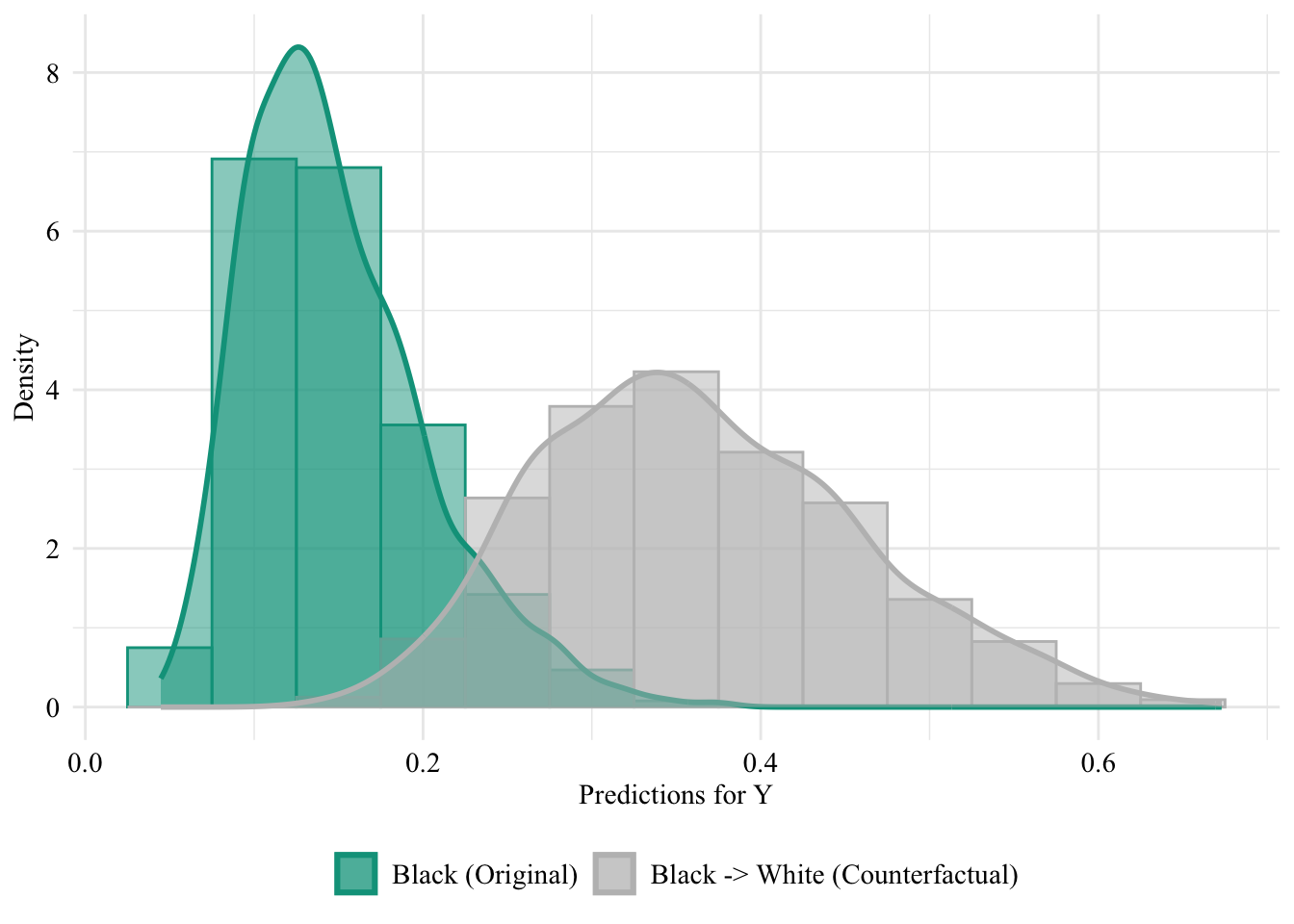
Now, we turn to the model that includes the sensitive attribute, i.e., the aware model.
We create a tibble with the factuals and the predictions by the aware model:
<- tibble (S = df_race_c$ S,S_origin = df_race_c$ S,X1 = df_race_c$ X1,X2 = df_race_c$ X2,Y = df_race_c$ Y,pred = pred_aware_all,type = "factual" |> mutate (id_indiv = row_number ())
<- |> mutate (S_origin = S) |> bind_rows (counterfactuals_aware_naive_black)
Codes used to create the Figure.
ggplot (|> mutate (group = case_when (== "Black" & S == "Black" ~ "Black (Original)" ,== "Black" & S == "White" ~ "Black -> White (Counterfactual)" ,== "White" & S == "White" ~ "White (Original)" group = factor (levels = c ("Black (Original)" , "Black -> White (Counterfactual)" , "White (Original)" aes (x = pred, fill = group, colour = group)+ geom_histogram (mapping = aes (y = after_stat (density)), alpha = 0.5 ,position = "identity" , binwidth = 0.05 + geom_density (alpha = 0.5 , linewidth = 1 ) + scale_fill_manual (NULL , values = c ("Black (Original)" = colours_all[["source" ]],"Black -> White (Counterfactual)" = colours_all[["naive" ]],"White (Original)" = colours_all[["reference" ]]+ facet_wrap (~ S) + labs (x = "Predictions for Y" ,y = "Density" + global_theme () + theme (legend.position = "bottom" )
Then, we focus on the distribution of predicted scores forcounterfactual of Black students and factuals of white students.
Codes used to create the Figure.
ggplot (data = aware_naive_black |> mutate (group = case_when (== "Black" & S == "Black" ~ "Black (Original)" ,== "Black" & S == "White" ~ "Black -> White (Counterfactual)" ,== "White" & S == "White" ~ "White (Original)" group = factor (levels = c ("Black (Original)" , "Black -> White (Counterfactual)" , "White (Original)" |> filter (S_origin == "Black" ),mapping = aes (x = pred, fill = group, colour = group)+ geom_histogram (mapping = aes (y = after_stat (density)), alpha = 0.5 , position = "identity" , binwidth = 0.05 + geom_density (alpha = 0.5 , linewidth = 1 ) + scale_fill_manual (NULL , values = c ("Black (Original)" = colours_all[["source" ]],"Black -> White (Counterfactual)" = colours_all[["naive" ]],"White (Original)" = colours_all[["reference" ]]+ scale_colour_manual (NULL , values = c ("Black (Original)" = colours_all[["source" ]],"Black -> White (Counterfactual)" = colours_all[["naive" ]],"White (Original)" = colours_all[["reference" ]]+ labs (x = "Predictions for Y" ,y = "Density" + global_theme () + theme (legend.position = "bottom" )
Saving Objects
save (counterfactuals_unaware_naive_black, file = "../data/counterfactuals_unaware_naive_black.rda" )save (counterfactuals_aware_naive_black, file = "../data/counterfactuals_aware_naive_black.rda" )


