This chapter uses fairadapt (Plečko and Meinshausen (2020 ) ) to make counterfactual inference. We obtain counterfactual values \(\boldsymbol{x}^\star\) for individuals from the protected group \(S=0\) . Then, we use the aware and unaware classifiers \(m(\cdot)\) (see Chapter 7 ) to make new predictions \(m(s=1,\boldsymbol{x}^\star)\) for individuals in the protected class, i.e., observations in \(\mathcal{D}_0\) .
In the article, we use three methods to create counterfactuals:
Naive approach (Chapter 8 )
Fairadapt (this chapter)
Multivariate optimal transport (Chapter 10 )
Sequential transport (the methodology we develop in the paper, see Chapter 11 ).
Required packages and definition of colours.
# Required packages---- library (tidyverse)library (fairadapt)# Graphs---- = font_title = 'Times New Roman' :: loadfonts (quiet = T)= 'plain' = 'plain' = 14 = 11 = 11 <- function () {theme_minimal () %+replace% theme (text = element_text (family = font_main, size = size_text, face = face_text),legend.text = element_text (family = font_main, size = legend_size),axis.text = element_text (size = size_text, face = face_text), plot.title = element_text (family = font_title, size = size_title, hjust = 0.5 plot.subtitle = element_text (hjust = 0.5 )# Seed set.seed (2025 )<- c ("source" = "#00A08A" ,"reference" = "#F2AD00" ,"naive" = "gray" ,"fairadapt" = '#D55E00'
Load Data and Classifier
We load the dataset where the sensitive attribute (\(S\) ) is the race, obtained Chapter 6.3 :
load ("../data/df_race.rda" )
We also load the dataset where the sensitive attribute is also the race, but where where the target variable (\(Y\) , ZFYA) is binary (1 if the student obtained a standardized first year average over the median, 0 otherwise). This dataset was saved in Chapter 7.5 :
load ("../data/df_race_c.rda" )
We also need the predictions made by the classifier (see Chapter 7 ):
# Predictions on train/test sets load ("../data/pred_aware.rda" )load ("../data/pred_unaware.rda" )# Predictions on the factuals, on the whole dataset load ("../data/pred_aware_all.rda" )load ("../data/pred_unaware_all.rda" )
We load the adjacency matrix that translates the assumed causal structure, obtained in Chapter 6.3 :
Counterfactuals with fairadapt
We adapt the code from Plečko, Bennett, and Meinshausen (2021 ) to handle the test set. This avoids estimating cumulative distribution and quantile functions on the test set, which would otherwise necessitate recalculating quantile regression functions for each new sample.
We do not need to adapt Y here, so we need to remove it from the adjacency matrix:
<- adj[- 4 ,- 4 ]
   S X1 X2
S  0  1  1
X1 0  0  1
X2 0  0  0
We create a dataset with the sensitive attribute and the two other predictors:
<- df_race_c |> select (S, X1, X2)
Let us have a look at the levels of our sensitive variable:
The reference class here consists of Black individuals.
Two configurations will be considered in turn:
The reference class consists of Black individuals, and FairAdapt will be used to obtain the counterfactual UGPA and LSAT scores for White individuals as if they had been Black.
The reference class consists of White individuals, and FairAdapt will be used to obtain the counterfactual UGPA and LSAT scores for Black individuals as if they had been White.
# White (factuals) --> Black (counterfactuals) <- fairadapt (~ ., train.data = df_race_fpt,prot.attr = "S" , adj.mat = adj_wo_Y,quant.method = linearQuants<- adaptedData (fpt_model_white)# Black (factuals) --> White (counterfactuals) $ S <- factor (df_race_fpt$ S, levels = c ("White" , "Black" ))<- fairadapt (~ ., train.data = df_race_fpt,prot.attr = "S" , adj.mat = adj_wo_Y,quant.method = linearQuants<- adaptedData (fpt_model_black)
Let us wrap up:
we have two predictive models for the FYA (above median = 1, or below median = 0):
unaware (without S)aware (with S) we have the counterfactual characteristics obtained with fairadapt in two situations depending on the reference class:
Black individuals as referenceWhite individuals as reference.
The predictive models will be used to compare predictions made using:
Raw characteristics (initial characteristics).Characteristics possibly altered through fairadapt for individuals who were not in the reference group (i.e., using counterfactuals).
Unaware Model
The predicted values using the initial characteristics (the factuals), for the unaware model are stored in the object pred_unaware_all. We put in a table the initial characteristics (factuals) and the prediction made by the unaware model:
<- tibble (S = df_race_c$ S,X1 = df_race_c$ X1,X2 = df_race_c$ X2,pred = pred_unaware_all,type = "factual" |> mutate (id_indiv = row_number ())
Let us save this dataset in a csv file (this file will be used to perform multivariate transport in python).
write.csv (file = "../data/factuals_unaware.csv" , row.names = FALSE
Let us get the predicted values for the counterfactuals, using the unaware model:
<- which (df_race_c$ S == "Black" )<- which (df_race_c$ S == "White" )<- pred_unaware$ model<- predict (newdata = adapt_df_black[ind_black, ], type = "response" <- predict (newdata = adapt_df_white[ind_white, ],type = "response"
We create a table with the counterfactual characteristics and the prediction by the unaware model:
<- as_tibble (adapt_df_black[ind_black, ]) |> mutate (S_origin = df_race_c$ S[ind_black],pred = pred_unaware_fpt_black,type = "counterfactual" ,id_indiv = ind_black<- as_tibble (adapt_df_white[ind_white, ]) |> mutate (S_origin = df_race_c$ S[ind_white],pred = pred_unaware_fpt_white,type = "counterfactual" ,id_indiv = ind_white
We merge the two datasets, factuals_unaware and counterfactuals_unaware_fpt in a single one.
# dataset with counterfactuals, for unaware model <- |> mutate (S_origin = S) |> bind_rows (counterfactuals_unaware_fpt_black)<- |> mutate (S_origin = S) |> bind_rows (counterfactuals_unaware_fpt_white)
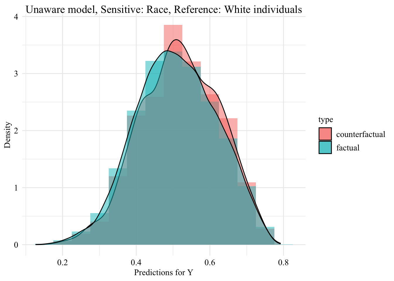
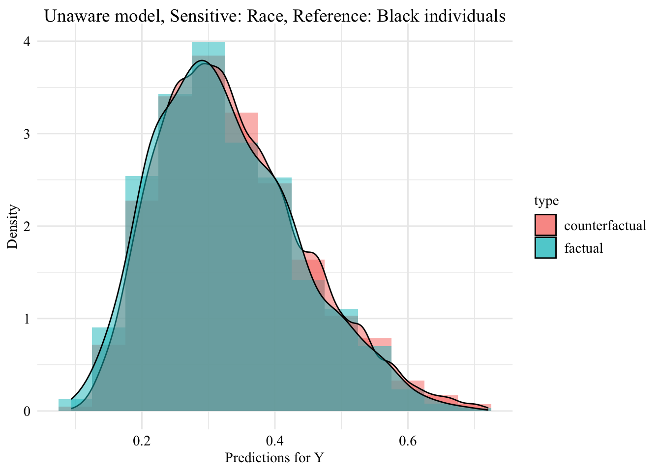
Now, we can visualize the distribution of the values predicted by the unaware model within each group defined by the sensitive attribute.
Codes used to create the Figure.
ggplot (data = unaware_fpt_black |> mutate (group = case_when (== "Black" & S == "Black" ~ "Black (Original)" ,== "Black" & S == "White" ~ "Black -> White (Counterfactual)" ,== "White" & S == "White" ~ "White (Original)" group = factor (levels = c ("Black (Original)" , "Black -> White (Counterfactual)" , "White (Original)" aes (x = pred, fill = group, colour = group)+ geom_histogram (mapping = aes (y = after_stat (density)), alpha = 0.5 , colour = NA ,position = "identity" , binwidth = 0.05 + geom_density (alpha = 0.3 , linewidth = 1 ) + facet_wrap (~ S) + scale_fill_manual (NULL , values = c ("Black (Original)" = colours_all[["source" ]],"Black -> White (Counterfactual)" = colours_all[["fairadapt" ]],"White (Original)" = colours_all[["reference" ]]+ scale_colour_manual (NULL , values = c ("Black (Original)" = colours_all[["source" ]],"Black -> White (Counterfactual)" = colours_all[["fairadapt" ]],"White (Original)" = colours_all[["reference" ]]+ labs (x = "Predictions for Y" ,y = "Density" + global_theme () + theme (legend.position = "bottom" )
Codes used to create the Figure.
ggplot (data = unaware_fpt_white |> mutate (group = case_when (== "White" & S == "White" ~ "White (Original)" ,== "White" & S == "Black" ~ "White -> Black (Counterfactual)" ,== "Black" & S == "Black" ~ "Black (Original)" group = factor (levels = c ("White (Original)" , "White -> Black (Counterfactual)" , "Black (Original)" aes (x = pred, fill = group, colour = group)+ geom_histogram (mapping = aes (y = after_stat (density)), alpha = 0.5 , colour = NA ,position = "identity" , binwidth = 0.05 + geom_density (alpha = 0.3 , linewidth = 1 ) + facet_wrap (~ S) + scale_fill_manual (NULL , values = c ("White (Original)" = colours_all[["source" ]],"White -> Black (Counterfactual)" = colours_all[["fairadapt" ]],"Black (Original)" = colours_all[["reference" ]]+ scale_colour_manual (NULL , values = c ("White (Original)" = colours_all[["source" ]],"White -> Black (Counterfactual)" = colours_all[["fairadapt" ]],"Black (Original)" = colours_all[["reference" ]]+ labs (x = "Predictions for Y" ,y = "Density" + global_theme () + theme (legend.position = "bottom" )
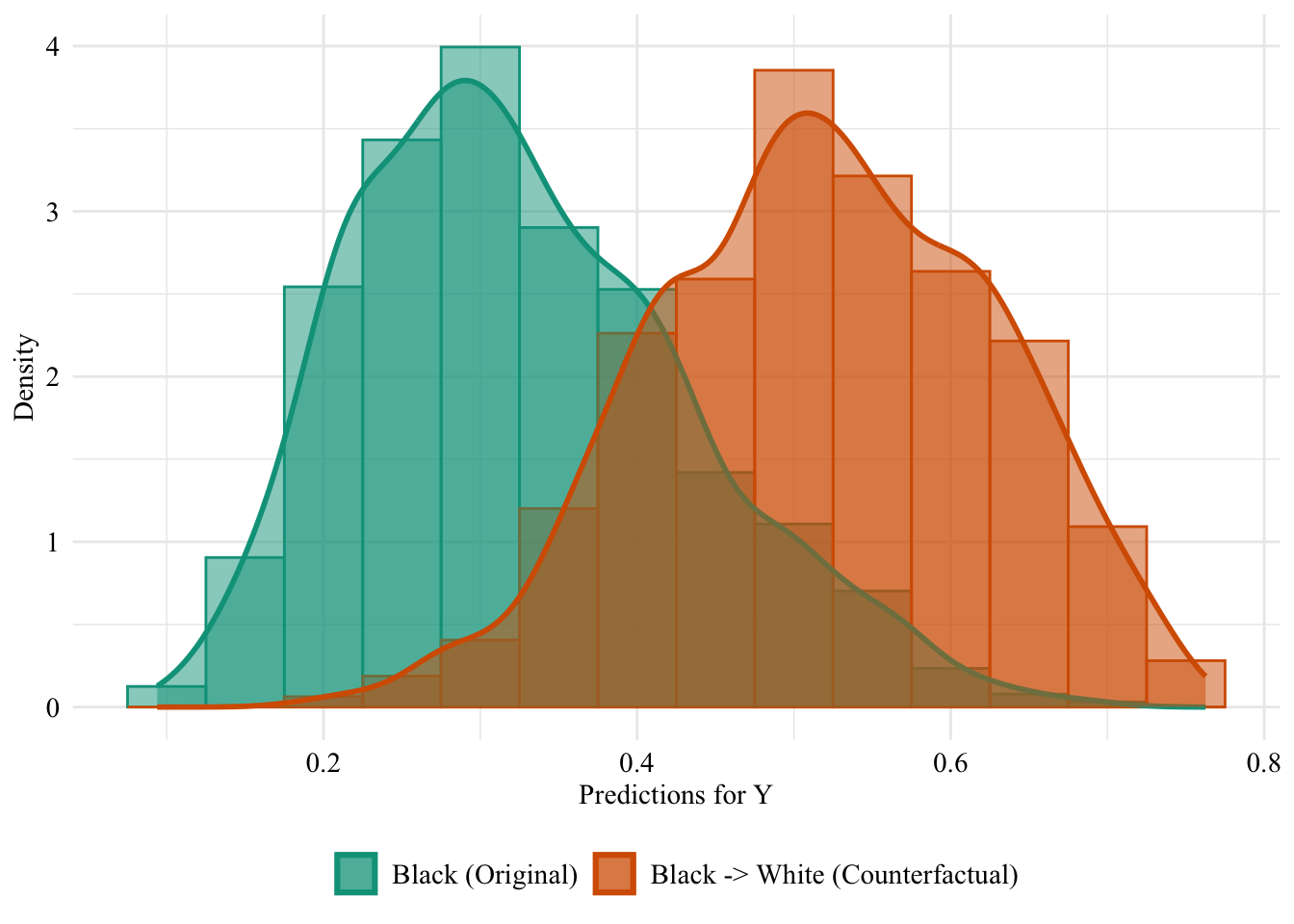
Then, we focus on the distribution of predicted scores for counterfactual of Black students and factuals of white students.
Codes used to create the Figure.
ggplot (data = unaware_fpt_black |> mutate (group = case_when (== "Black" & S == "Black" ~ "Black (Original)" ,== "Black" & S == "White" ~ "Black -> White (Counterfactual)" ,== "White" & S == "White" ~ "White (Original)" group = factor (levels = c ("Black (Original)" , "Black -> White (Counterfactual)" , "White (Original)" |> filter (S_origin == "Black" ),mapping = aes (x = pred, fill = group, colour = group)+ geom_histogram (mapping = aes (y = after_stat (density)), alpha = 0.5 , position = "identity" , binwidth = 0.05 + geom_density (alpha = 0.5 , linewidth = 1 ) + scale_fill_manual (NULL , values = c ("Black (Original)" = colours_all[["source" ]],"Black -> White (Counterfactual)" = colours_all[["fairadapt" ]],"White (Original)" = colours_all[["reference" ]]+ scale_colour_manual (NULL , values = c ("Black (Original)" = colours_all[["source" ]],"Black -> White (Counterfactual)" = colours_all[["fairadapt" ]],"White (Original)" = colours_all[["reference" ]]+ labs (x = "Predictions for Y" ,y = "Density" + global_theme () + theme (legend.position = "bottom" )
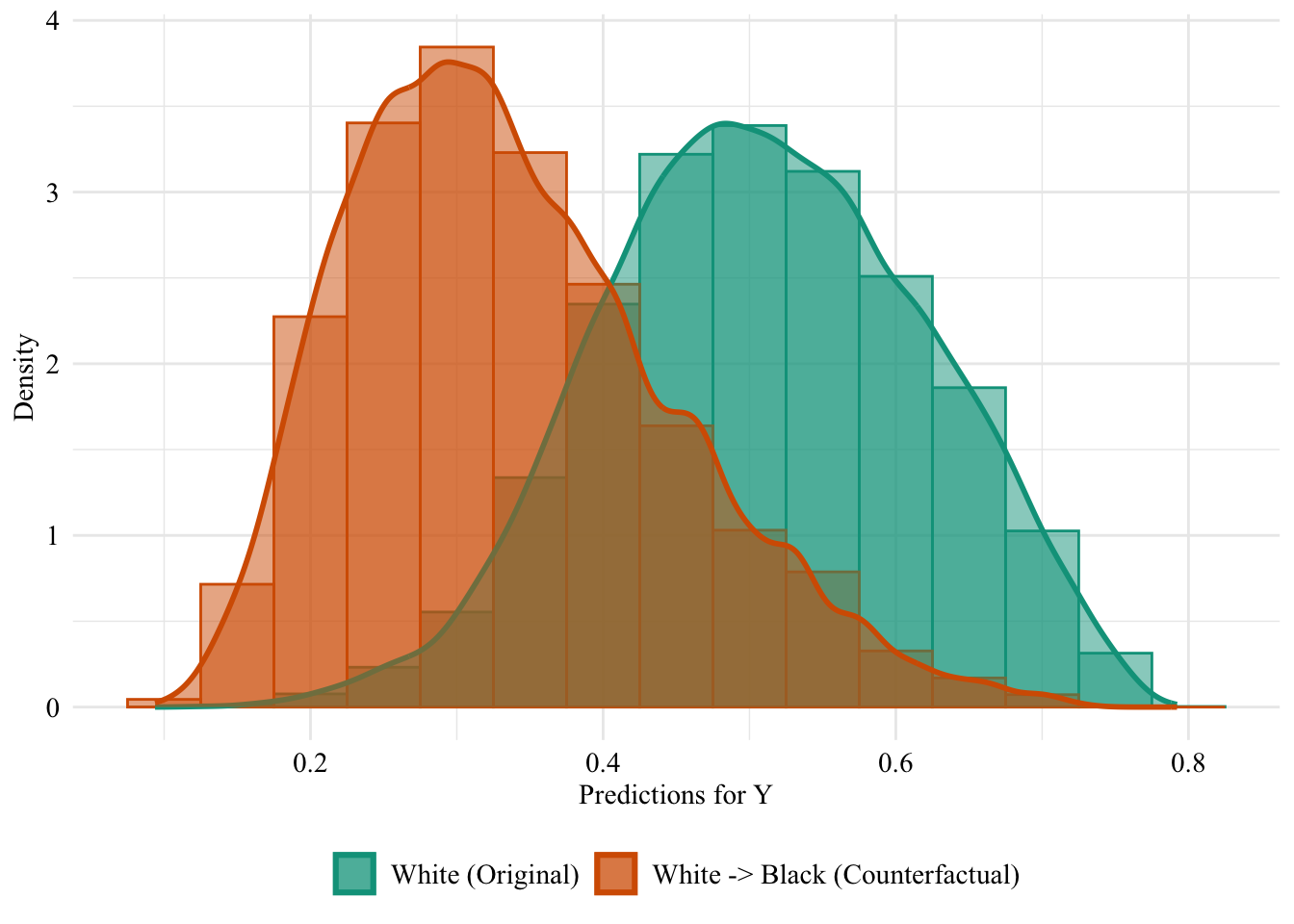
Codes used to create the Figure.
ggplot (data = unaware_fpt_white |> mutate (group = case_when (== "White" & S == "White" ~ "White (Original)" ,== "White" & S == "Black" ~ "White -> Black (Counterfactual)" ,== "Black" & S == "Black" ~ "Black (Original)" group = factor (levels = c ("White (Original)" , "White -> Black (Counterfactual)" , "Black (Original)" |> filter (S_origin == "White" ),mapping = aes (x = pred, fill = group, colour = group)) + geom_histogram (mapping = aes (y = after_stat (density)), alpha = 0.5 , position = "identity" , binwidth = 0.05 + geom_density (alpha = 0.5 , linewidth = 1 ) + scale_fill_manual (NULL , values = c ("White (Original)" = colours_all[["source" ]],"White -> Black (Counterfactual)" = colours_all[["fairadapt" ]]+ scale_colour_manual (NULL , values = c ("White (Original)" = colours_all[["source" ]],"White -> Black (Counterfactual)" = colours_all[["fairadapt" ]]+ labs (x = "Predictions for Y" ,y = "Density" + global_theme () + theme (legend.position = "bottom" )
Aware Model
Now, we turn to the model that includes the sensitive attribute, i.e., the aware model.
The predicted values by the model, on the initial characteristics (on the factuals) are stored in the pred_aware_all object.
We create a tibble with the factuals and the predictions by the aware model:
<- tibble (S = df_race$ S,X1 = df_race$ X1,X2 = df_race$ X2,pred = pred_aware_all,type = "factual" |> mutate (id_indiv = row_number ())
Let us save this table in a CSV file (this file will be used to perform multivariate transport in python):
write.csv (file = "../data/factuals_aware.csv" , row.names = FALSE
Let us get the predicted values for the counterfactuals, using the aware model:
<- pred_aware$ model<- predict (newdata = adapt_df_black[ind_black, ], type = "response" <- predict (newdata = adapt_df_white[ind_white, ],type = "response"
We create a table with the counterfactual characteristics and the prediction by the aware model:
<- as_tibble (adapt_df_black[ind_black, ]) |> mutate (S_origin = df_race_c$ S[ind_black],pred = pred_aware_fpt_black,type = "counterfactual" ,id_indiv = ind_black<- as_tibble (adapt_df_white[ind_white, ]) |> mutate (S_origin = df_race_c$ S[ind_white],pred = pred_aware_fpt_white,type = "counterfactual" ,id_indiv = ind_white
We merge the two datasets, factuals_unaware and counterfactuals_aware_fpt in a single one.
# dataset with counterfactuals, for aware model <- |> mutate (S_origin = S) |> bind_rows (counterfactuals_aware_fpt_black)<- |> mutate (S_origin = S) |> bind_rows (counterfactuals_aware_fpt_white)
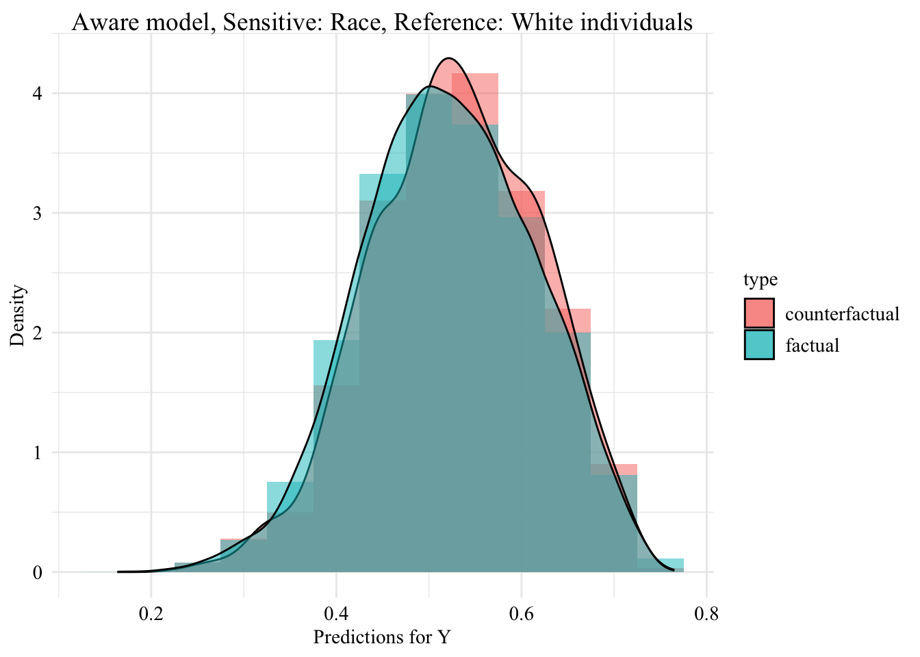
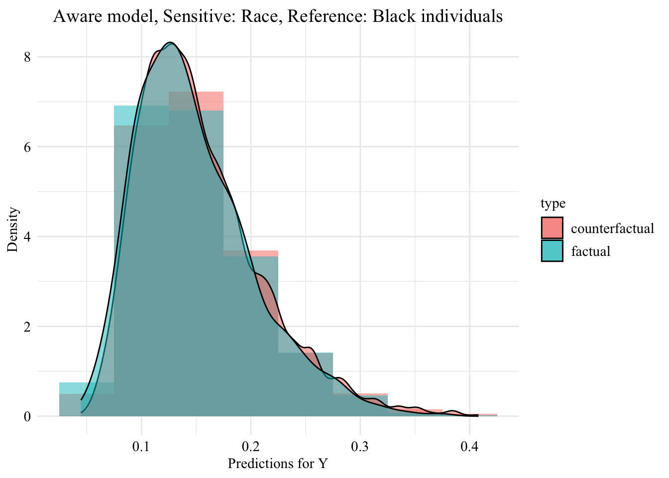
Now, we can visualize the distribution of the values predicted by the unaware model within each group defined by the sensitive attribute.
Codes used to create the Figure.
ggplot (data = aware_fpt_black |> mutate (group = case_when (== "Black" & S == "Black" ~ "Black (Original)" ,== "Black" & S == "White" ~ "Black -> White (Counterfactual)" ,== "White" & S == "White" ~ "White (Original)" group = factor (levels = c ("Black (Original)" , "Black -> White (Counterfactual)" , "White (Original)" aes (x = pred, fill = group, colour = group)+ geom_histogram (mapping = aes (y = after_stat (density)), alpha = 0.5 , colour = NA ,position = "identity" , binwidth = 0.05 + geom_density (alpha = 0.3 , linewidth = 1 ) + facet_wrap (~ S) + scale_fill_manual (NULL , values = c ("Black (Original)" = colours_all[["source" ]],"Black -> White (Counterfactual)" = colours_all[["fairadapt" ]],"White (Original)" = colours_all[["reference" ]]+ scale_colour_manual (NULL , values = c ("Black (Original)" = colours_all[["source" ]],"Black -> White (Counterfactual)" = colours_all[["fairadapt" ]],"White (Original)" = colours_all[["reference" ]]+ labs (x = "Predictions for Y" ,y = "Density" + global_theme () + theme (legend.position = "bottom" )
Codes used to create the Figure.
ggplot (data = aware_fpt_white |> mutate (group = case_when (== "White" & S == "White" ~ "White (Original)" ,== "White" & S == "Black" ~ "White -> Black (Counterfactual)" ,== "Black" & S == "Black" ~ "Black (Original)" group = factor (levels = c ("White (Original)" , "White -> Black (Counterfactual)" , "Black (Original)" aes (x = pred, fill = group, colour = group)+ geom_histogram (mapping = aes (y = after_stat (density)), alpha = 0.5 , colour = NA ,position = "identity" , binwidth = 0.05 + geom_density (alpha = 0.3 , linewidth = 1 ) + facet_wrap (~ S) + scale_fill_manual (NULL , values = c ("White (Original)" = colours_all[["source" ]],"White -> Black (Counterfactual)" = colours_all[["fairadapt" ]],"Black (Original)" = colours_all[["reference" ]]+ scale_colour_manual (NULL , values = c ("White (Original)" = colours_all[["source" ]],"White -> Black (Counterfactual)" = colours_all[["fairadapt" ]],"Black (Original)" = colours_all[["reference" ]]+ labs (x = "Predictions for Y" ,y = "Density" + global_theme () + theme (legend.position = "bottom" )
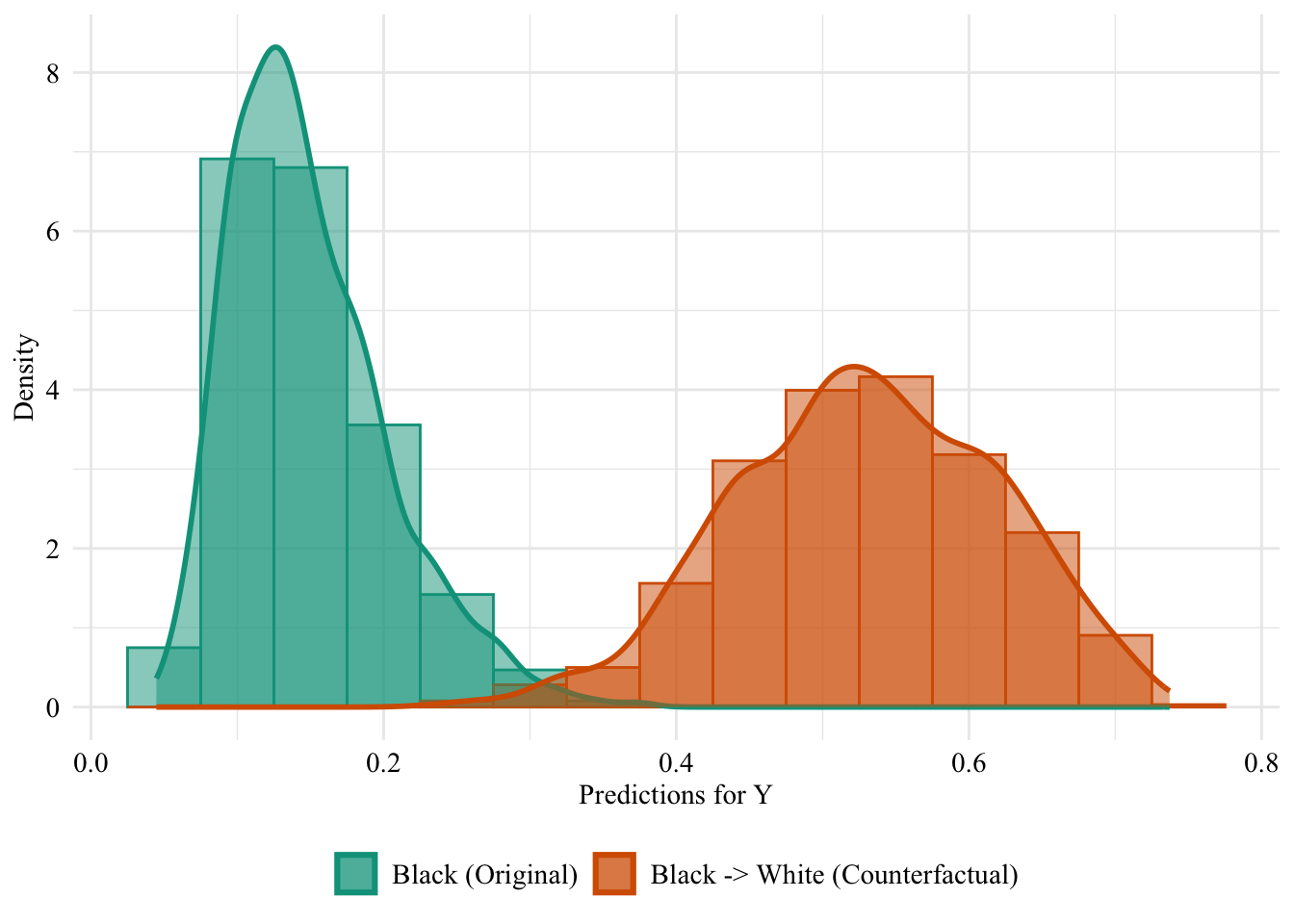
Then, we focus on the distribution of predicted scores for counterfactual of Black students and factuals of white students.
Codes used to create the Figure.
ggplot (data = aware_fpt_black |> mutate (group = case_when (== "Black" & S == "Black" ~ "Black (Original)" ,== "Black" & S == "White" ~ "Black -> White (Counterfactual)" ,== "White" & S == "White" ~ "White (Original)" group = factor (levels = c ("Black (Original)" , "Black -> White (Counterfactual)" , "White (Original)" |> filter (S_origin == "Black" ),mapping = aes (x = pred, fill = group, colour = group)+ geom_histogram (mapping = aes (y = after_stat (density)), alpha = 0.5 , position = "identity" , binwidth = 0.05 + geom_density (alpha = 0.5 , linewidth = 1 ) + scale_fill_manual (NULL , values = c ("Black (Original)" = colours_all[["source" ]],"Black -> White (Counterfactual)" = colours_all[["fairadapt" ]],"White (Original)" = colours_all[["reference" ]]+ scale_colour_manual (NULL , values = c ("Black (Original)" = colours_all[["source" ]],"Black -> White (Counterfactual)" = colours_all[["fairadapt" ]],"White (Original)" = colours_all[["reference" ]]+ labs (x = "Predictions for Y" ,y = "Density" + global_theme () + theme (legend.position = "bottom" )
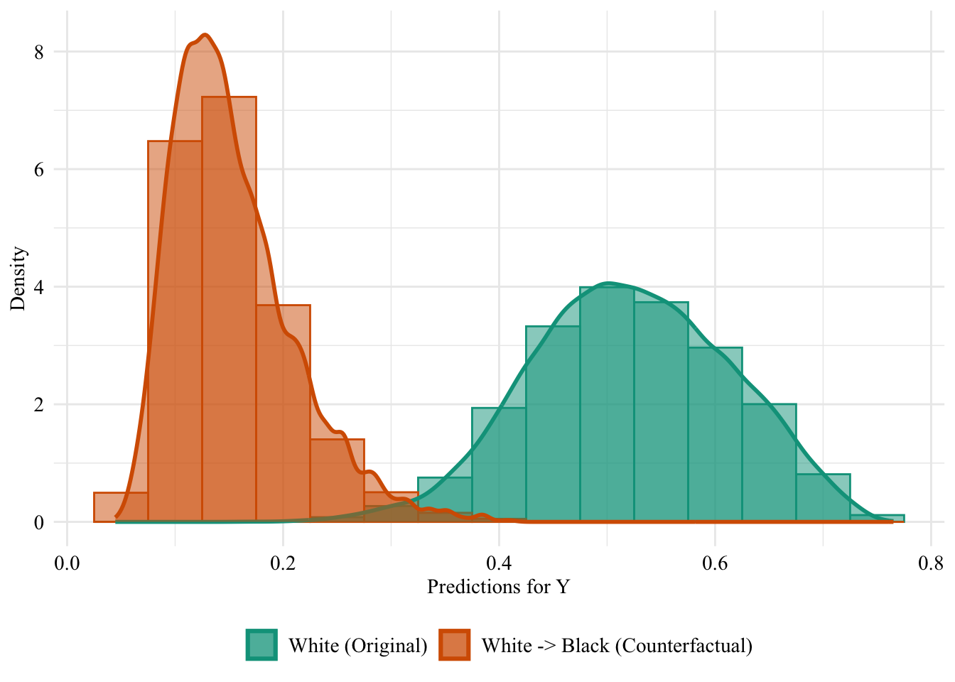
Codes used to create the Figure.
ggplot (data = aware_fpt_white |> mutate (group = case_when (== "White" & S == "White" ~ "White (Original)" ,== "White" & S == "Black" ~ "White -> Black (Counterfactual)" ,== "Black" & S == "Black" ~ "Black (Original)" group = factor (levels = c ("White (Original)" , "White -> Black (Counterfactual)" , "Black (Original)" |> filter (S_origin == "White" ),mapping = aes (x = pred, fill = group, colour = group)+ geom_histogram (mapping = aes (y = after_stat (density)), alpha = 0.5 , position = "identity" , binwidth = 0.05 + geom_density (alpha = 0.5 , linewidth = 1 ) + scale_fill_manual (NULL , values = c ("White (Original)" = colours_all[["source" ]],"White -> Black (Counterfactual)" = colours_all[["fairadapt" ]]+ scale_colour_manual (NULL , values = c ("White (Original)" = colours_all[["source" ]],"White -> Black (Counterfactual)" = colours_all[["fairadapt" ]]+ labs (x = "Predictions for Y" ,y = "Density" + global_theme () + theme (legend.position = "bottom" )
Comparison for Two Individuals
Let us focus on two individuals: the 24th (Black) and the 25th (White) of the dataset.
<- factuals_unaware |> filter (id_indiv %in% c (24 , 25 )))
# A tibble: 2 × 6
  S        X1    X2  pred type    id_indiv
  <fct> <dbl> <dbl> <dbl> <chr>      <int>
1 Black   2.8    29 0.300 factual       24
2 White   2.8    34 0.382 factual       25
The characteristics of these two individuals would be, according to what was estimated using fairadapt, if the reference group was the one in which they do not belong:
<- |> filter (id_indiv %in% c (24 )) |> bind_rows (|> filter (id_indiv %in% c (25 ))
# A tibble: 2 × 7
     X2 S        X1 S_origin  pred type           id_indiv
  <dbl> <fct> <dbl> <fct>    <dbl> <chr>             <int>
1  37.6 White  3.25 Black    0.509 counterfactual       24
2  26   Black  2.5  White    0.225 counterfactual       25
We put the factuals and counterfactuals in a single table:
<- bind_rows (
# A tibble: 4 × 7
  S        X1    X2  pred type           id_indiv S_origin
  <fct> <dbl> <dbl> <dbl> <chr>             <int> <fct>
1 Black  2.8   29   0.300 factual              24 <NA>
2 White  2.8   34   0.382 factual              25 <NA>
3 White  3.25  37.6 0.509 counterfactual       24 Black
4 Black  2.5   26   0.225 counterfactual       25 White
The difference between the counterfactual and the factual for these two individuals:
|> select (id_indiv , type, pred) |> pivot_wider (names_from = type, values_from = pred) |> mutate (diff_fpt = counterfactual - factual)
# A tibble: 2 × 4
  id_indiv factual counterfactual diff_fpt
     <int>   <dbl>          <dbl>    <dbl>
1       24   0.300          0.509    0.209
2       25   0.382          0.225   -0.157
We apply the same procedure with the aware model:
<- bind_rows (|> filter (id_indiv %in% c (24 , 25 )),|> filter (id_indiv == 24 ),|> filter (id_indiv == 25 )
# A tibble: 4 × 7
  S        X1    X2   pred type           id_indiv S_origin
  <fct> <dbl> <dbl>  <dbl> <chr>             <int> <fct>
1 Black  2.8   29   0.133  factual              24 <NA>
2 White  2.8   34   0.413  factual              25 <NA>
3 White  3.25  37.6 0.522  counterfactual       24 Black
4 Black  2.5   26   0.0991 counterfactual       25 White
The difference between the counterfactual and the factual for these two individuals, when using the aware model:
|> select (id_indiv , type, pred) |> pivot_wider (names_from = type, values_from = pred) |> mutate (diff = counterfactual - factual)
# A tibble: 2 × 4
  id_indiv factual counterfactual   diff
     <int>   <dbl>          <dbl>  <dbl>
1       24   0.133         0.522   0.389
2       25   0.413         0.0991 -0.314
Saving Objects
save (factuals_unaware, file = "../data/factuals_unaware.rda" )save (factuals_aware, file = "../data/factuals_aware.rda" )save (counterfactuals_unaware_fpt_black, file = "../data/counterfactuals_unaware_fpt_black.rda" )save (counterfactuals_aware_fpt_black, file = "../data/counterfactuals_aware_fpt_black.rda" )
Plečko, Drago, Nicolas Bennett, and Nicolai Meinshausen. 2021. “Fairadapt: Causal Reasoning for Fair Data Pre-Processing.” arXiv Preprint arXiv:2110.10200 .
Plečko, Drago, and Nicolai Meinshausen. 2020. “Fair Data Adaptation with Quantile Preservation.” Journal of Machine Learning Research 21 (242): 1–44.