This chapter uses multivariate optimal transport (De Lara et al. (2024 ) ) to make counterfactual inference. We obtain counterfactual values \(\boldsymbol{x}^\star\) for individuals from the protected group \(S=0\) . Then, we use the aware and unaware classifiers \(m(\cdot)\) (see Chapter 7 ) to make new predictions \(m(s=1,\boldsymbol{x}^\star)\) for individuals in the protected class, i.e., observations in \(\mathcal{D}_0\) .
In the article, we use three methods to create counterfactuals:
Naive approach (Chapter 8 )
Fairadapt (Chapter 9 )
Multivariate optimal transport (this chapter)
Sequential transport (the methodology we develop in the paper, see Chapter 11 ).
Required packages and definition of colours.
# Required packages---- library (tidyverse)library (fairadapt)# Graphs---- = font_title = 'Times New Roman' :: loadfonts (quiet = T)= 'plain' = 'plain' = 14 = 11 = 11 <- function () {theme_minimal () %+replace% theme (text = element_text (family = font_main, size = size_text, face = face_text),legend.text = element_text (family = font_main, size = legend_size),axis.text = element_text (size = size_text, face = face_text), plot.title = element_text (family = font_title, size = size_title, hjust = 0.5 plot.subtitle = element_text (hjust = 0.5 ),legend.position = "bottom" # Seed set.seed (2025 )library (devtools)load_all ("../seqtransfairness/" )<- c ("source" = "#00A08A" ,"reference" = "#F2AD00" ,"naive" = "gray" ,"fairadapt" = '#D55E00' ,"ot" = "#56B4E9"
Load Data and Classifier
We load the dataset where the sensitive attribute (\(S\) ) is the race, obtained Chapter 6.3 :
load ("../data/df_race.rda" )
We also load the dataset where the sensitive attribute is also the race, but where where the target variable (\(Y\) , ZFYA) is binary (1 if the student obtained a standardized first year average over the median, 0 otherwise). This dataset was saved in Chapter 7.5 :
load ("../data/df_race_c.rda" )
We also need the predictions made by the classifier (see Chapter 7 ):
# Predictions on train/test sets load ("../data/pred_aware.rda" )load ("../data/pred_unaware.rda" )# Predictions on the factuals, on the whole dataset load ("../data/pred_aware_all.rda" )load ("../data/pred_unaware_all.rda" )
Counterfactuals with Multivariate Optimal Transport
We apply multivariate optimal transport (OT), following the methodology developed in De Lara et al. (2024 ) . Note that with OT, it is not possible to handle new cases. Counterfactuals will only be calculated on the train set.
The codes are run in python. We use the {reticulate} R package to call python in this notebook.
library (reticulate)use_virtualenv ("~/quarto-python-env" , required = TRUE )# reticulate::install_miniconda(force = TRUE) # py_install("POT")
Some libraries need to be loaded (including POT called ot)
import otimport pandas as pdimport numpy as npimport matplotlib.pyplot as plimport ot.plot
The data with the factuals need to be loaded:
= pd.read_csv('../data/factuals_aware.csv' )= pd.read_csv('../data/factuals_unaware.csv' )
= df_aware.drop(columns= ['pred' , 'type' , 'id_indiv' ])
       S   X1    X2
0  White  3.1  39.0
1  White  3.0  36.0
2  White  3.1  30.0
3  White  3.4  37.0
4  White  3.6  30.5
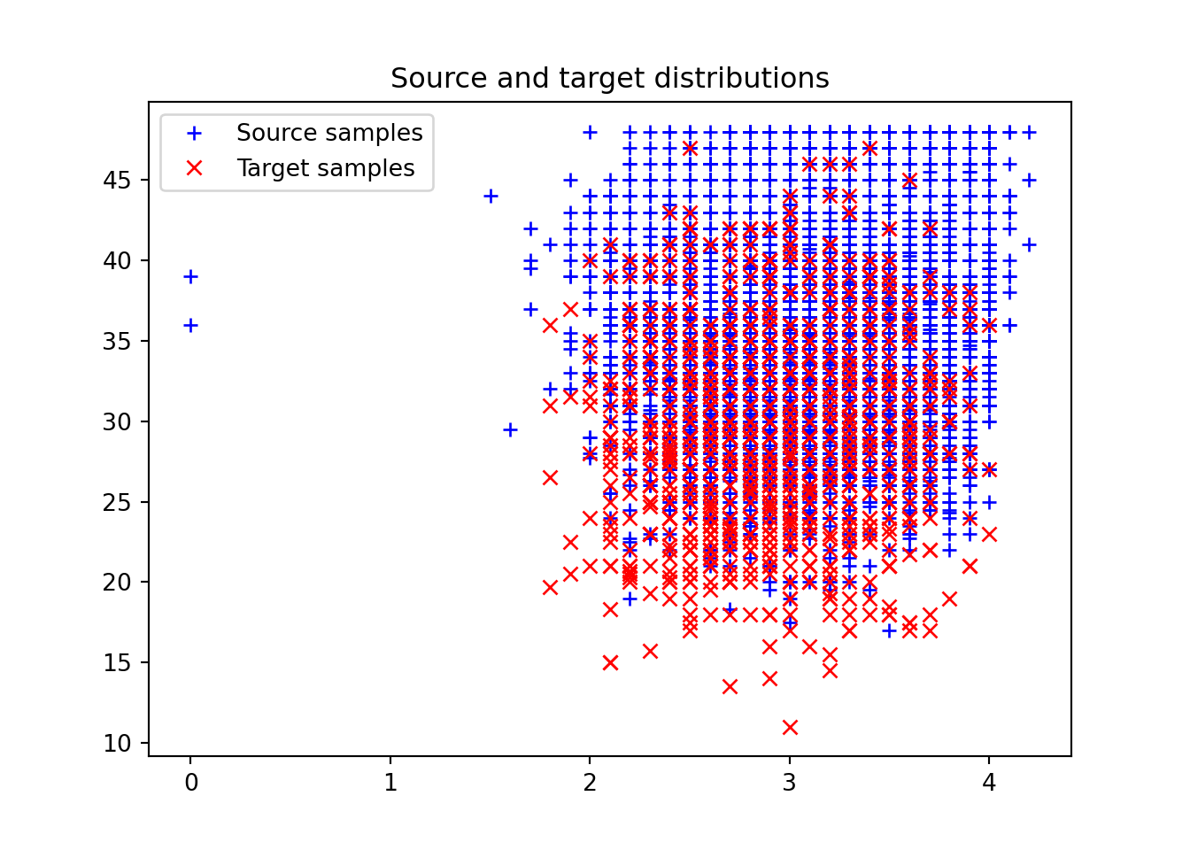
= x_S[x_S['S' ] == 'White' ]= x_white.drop(columns= ['S' ])= x_S[x_S['S' ] == 'Black' ]= x_black.drop(columns= ['S' ])= len (x_white)= len (x_black)# Uniform weights = (1 / n_white)* np.ones(n_white)= (1 / n_black)* np.ones(n_black)
Cost matrix between both distributions:
= x_white.to_numpy()= x_black.to_numpy()= ot.dist(x_white, x_black)
1 )0 ], x_white[:, 1 ], '+b' , label= 'Source samples' )0 ], x_black[:, 1 ], 'xr' , label= 'Target samples' )= 0 )'Source and target distributions' )
2 )= 'nearest' )'Cost matrix C' )
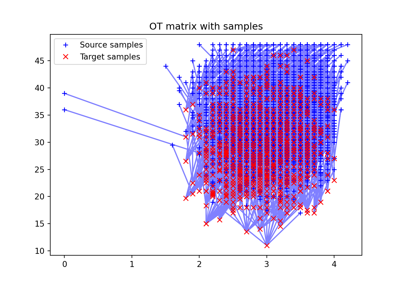
The transport plan: white –> black
= ot.emd(w_white, w_black, C, numItermax= 1e8 )= pi_white_black.T
= np.sum (pi_white_black, axis= 1 )* n_white
array([1., 1., 1., ..., 1., 1., 1.], shape=(18285,))
= np.sum (pi_black_white, axis= 1 )* n_black
array([1., 1., 1., ..., 1., 1., 1.], shape=(1282,))
3 )= 'nearest' )'OT matrix pi_white_black' )4 )= [.5 , .5 , 1 ])0 ], x_white[:, 1 ], '+b' , label= 'Source samples' )0 ], x_black[:, 1 ], 'xr' , label= 'Target samples' )= 0 )'OT matrix with samples' )
= n_white* pi_white_black@ x_black
array([[ 2.7, 31. ],
       [ 2.7, 28. ],
       [ 2.6, 21. ],
       ...,
       [ 3.9, 28. ],
       [ 2.5, 22. ],
       [ 3. , 19. ]], shape=(18285, 2))
= n_black* pi_black_white@ x_white
array([[ 3.2       , 37.58851518],
       [ 3.28565491, 28.02103363],
       [ 2.95793273, 32.14022423],
       ...,
       [ 3.28597758, 33.        ],
       [ 2.65092152, 41.43910309],
       [ 2.75152858, 36.        ]], shape=(1282, 2))
= x_S.drop(columns= ['S' ])'S' ] == 'White' ] = transformed_x_white'S' ] == 'Black' ] = transformed_x_black
    X1    X2
0  2.7  31.0
1  2.7  28.0
2  2.6  21.0
3  3.1  28.0
4  3.2  21.0
array([[ 2.7, 31. ],
       [ 2.7, 28. ],
       [ 2.6, 21. ],
       ...,
       [ 3.9, 28. ],
       [ 2.5, 22. ],
       [ 3. , 19. ]], shape=(18285, 2))
Lastly, we export the results in a CSV file:
= '../data/counterfactuals_ot.csv' = False )
Let us get back to R, and load the results.
<- read_csv ('../data/counterfactuals_ot.csv' ) |> mutate (id_indiv = row_number ())
We add the sensitive attribute to the dataset (Black individuals become White, and conversely):
<- df_race_c |> mutate (S_star = case_when (== "Black" ~ "White" ,== "White" ~ "Black" ,TRUE ~ "Error" |> pull ("S_star" )<- counterfactuals_ot |> mutate (S_origin = df_race_c$ S,S = S_star
<- |> filter (S_origin == "Black" ) |> bind_rows (|> select (- Y) |> mutate (id_indiv = row_number (),S_origin = S,|> filter (S == "White" )|> arrange (id_indiv)<- |> filter (S_origin == "White" ) |> bind_rows (|> select (- Y) |> mutate (id_indiv = row_number (),S_origin = S,|> filter (S == "Black" )|> arrange (id_indiv)
We consider Black individuals (minority group) to be the source group. Let us make prediction with the unaware model, then with the aware model on the counterfactuals obtained with OT.
<- pred_unaware$ model<- predict (newdata = counterfactuals_ot_black, type = "response" <- counterfactuals_ot_black |> mutate (pred = pred_unaware_ot_black, type = "counterfactual" )
If, instead, the source group is White:
<- predict (newdata = counterfactuals_ot_white, type = "response" <- counterfactuals_ot_white |> mutate (pred = pred_unaware_ot_white, type = "counterfactual" )
With the aware model, if Black is the source group:
<- pred_aware$ model<- predict (newdata = counterfactuals_ot_black, type = "response" <- counterfactuals_ot_black |> mutate (pred = pred_aware_ot_black, type = "counterfactual" )
If, instead, the source group is White:
<- predict (newdata = counterfactuals_ot_white, type = "response" <- counterfactuals_ot_white |> mutate (pred = pred_aware_ot_white, type = "counterfactual" )
Next, we can compare predicted scores for both type of model and on the source group.
Unaware Model
The predicted values using the initial characteristics (the factuals), for the unaware model are stored in the object pred_unaware_all. We put in a table the initial characteristics (factuals) and the prediction made by the unaware model:
<- tibble (S = df_race_c$ S,S_origin = df_race_c$ S,X1 = df_race_c$ X1,X2 = df_race_c$ X2,Y = df_race_c$ Y,pred = pred_unaware_all,type = "factual" |> mutate (id_indiv = row_number ())
We bind together the predictions made with the observed values and those made with the counterfactual values.
<- |> mutate (S_origin = S) |> bind_rows (counterfactuals_unaware_ot_black)<- |> mutate (S_origin = S) |> bind_rows (counterfactuals_unaware_ot_white)
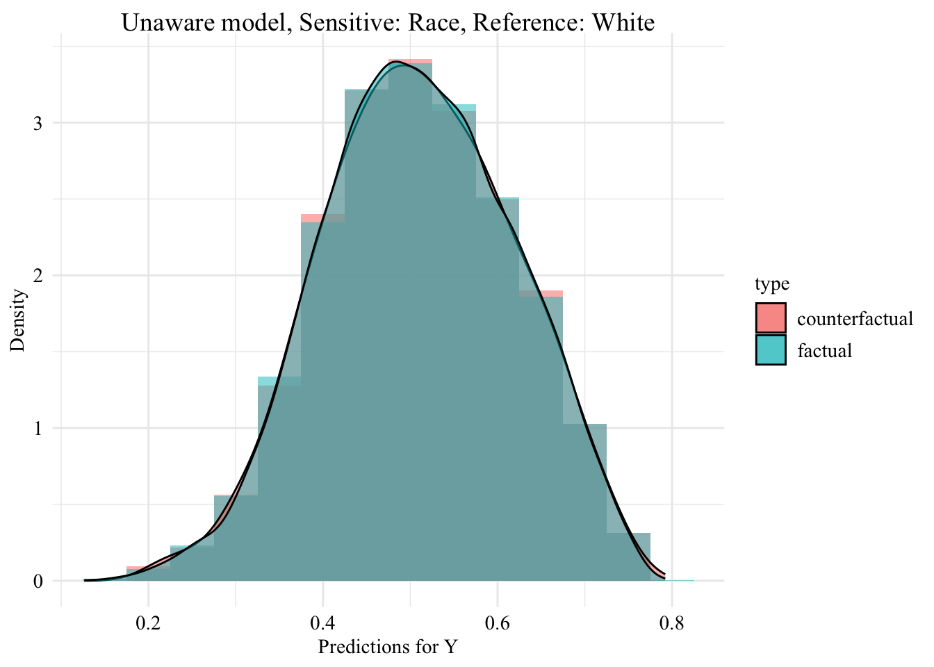
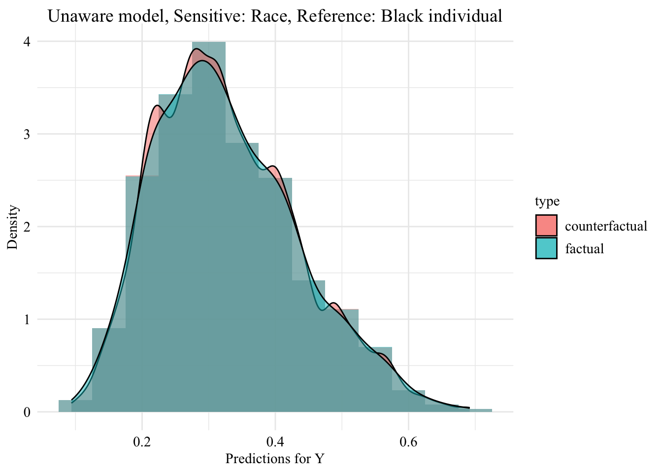
Now, we can visualize the distribution of the values predicted by the unaware model within each group defined by the sensitive attribute.
Codes used to create the Figure.
ggplot (data = unaware_ot_black |> mutate (group = case_when (== "Black" & S == "Black" ~ "Black (Original)" ,== "Black" & S == "White" ~ "Black -> White (Counterfactual)" ,== "White" & S == "White" ~ "White (Original)" group = factor (levels = c ("Black (Original)" , "Black -> White (Counterfactual)" , "White (Original)" aes (x = pred, fill = group, colour = group)+ geom_histogram (mapping = aes (y = after_stat (density)), alpha = 0.5 , colour = NA ,position = "identity" , binwidth = 0.05 + geom_density (alpha = 0.3 , linewidth = 1 ) + facet_wrap (~ S) + scale_fill_manual (NULL , values = c ("Black (Original)" = colours_all[["source" ]],"Black -> White (Counterfactual)" = colours_all[["ot" ]],"White (Original)" = colours_all[["reference" ]]+ scale_colour_manual (NULL , values = c ("Black (Original)" = colours_all[["source" ]],"Black -> White (Counterfactual)" = colours_all[["ot" ]],"White (Original)" = colours_all[["reference" ]]+ labs (title = "Unaware model, Sensitive: Race, Reference: White individuals" ,x = "Predictions for Y" ,y = "Density" + global_theme () + theme (legend.position = "bottom" )
Codes used to create the Figure.
ggplot (data = unaware_ot_white |> mutate (group = case_when (== "White" & S == "White" ~ "White (Original)" ,== "White" & S == "Black" ~ "White -> Black (Counterfactual)" ,== "Black" & S == "Black" ~ "Black (Original)" group = factor (levels = c ("White (Original)" , "White -> Black (Counterfactual)" , "Black (Original)" aes (x = pred, fill = group, colour = group)+ geom_histogram (mapping = aes (y = after_stat (density)), alpha = 0.5 , colour = NA ,position = "identity" , binwidth = 0.05 + geom_density (alpha = 0.3 , linewidth = 1 ) + facet_wrap (~ S) + scale_fill_manual (NULL , values = c ("White (Original)" = colours_all[["source" ]],"White -> Black (Counterfactual)" = colours_all[["ot" ]],"Black (Original)" = colours_all[["reference" ]]+ scale_colour_manual (NULL , values = c ("White (Original)" = colours_all[["source" ]],"White -> Black (Counterfactual)" = colours_all[["ot" ]],"Black (Original)" = colours_all[["reference" ]]+ labs (title = "Unaware model, Sensitive: Race, Reference: Black individuals" ,x = "Predictions for Y" ,y = "Density" + global_theme () + theme (legend.position = "bottom" )
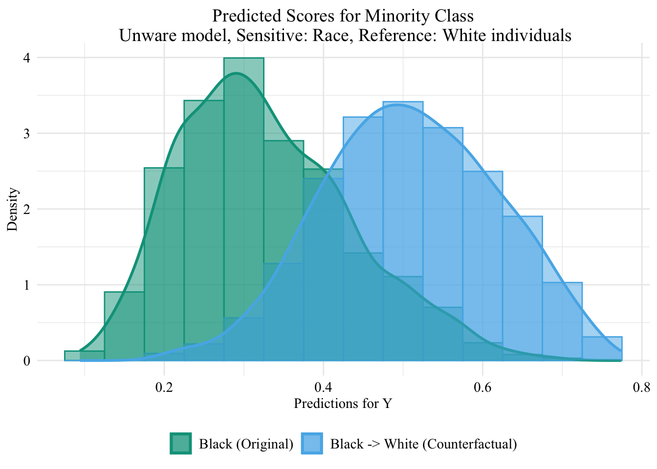
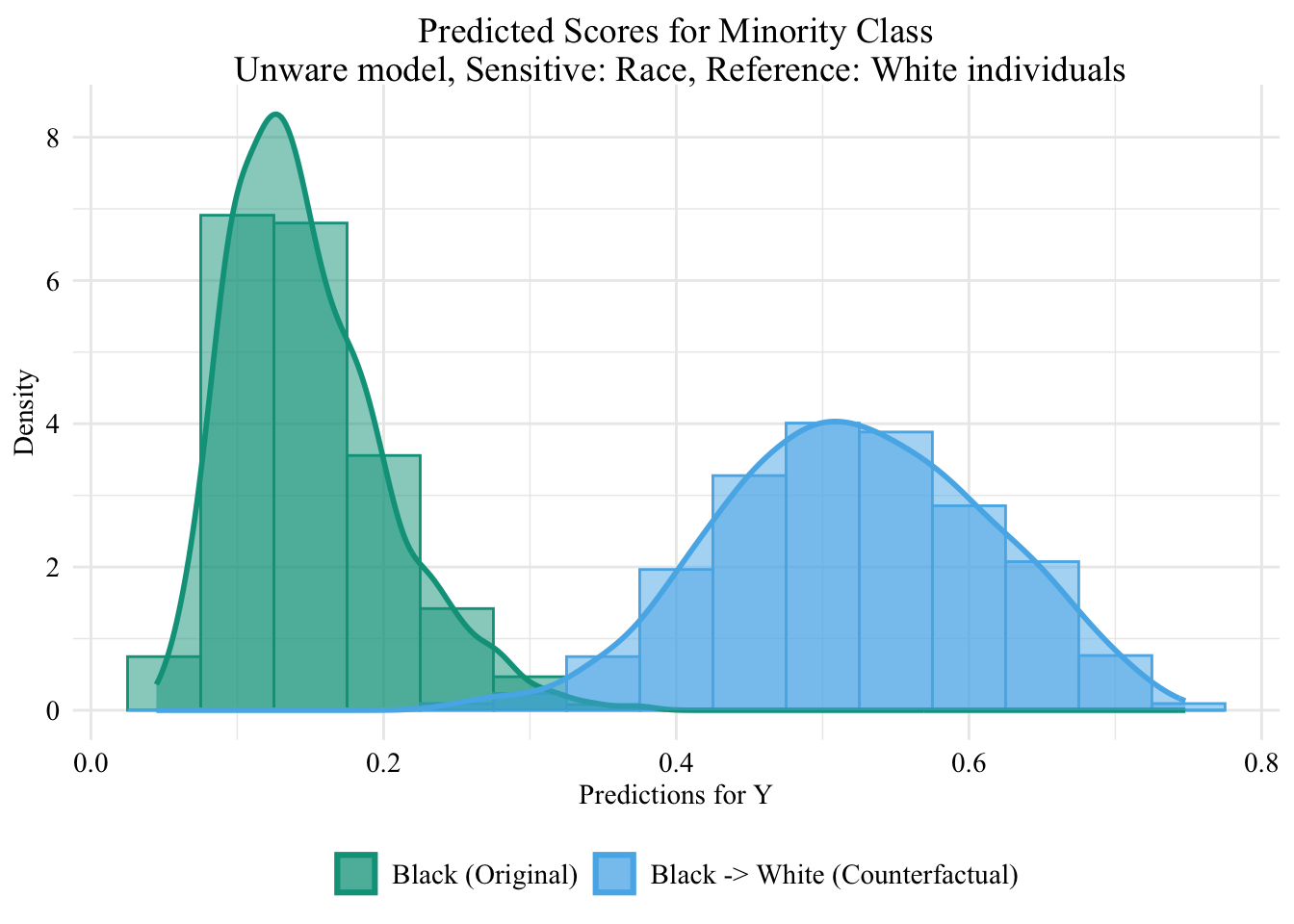
Then, we focus on the distribution of predicted scores forcounterfactual of Black students and factuals of white students.
Codes used to create the Figure.
ggplot (data = unaware_ot_black |> mutate (group = case_when (== "Black" & S == "Black" ~ "Black (Original)" ,== "Black" & S == "White" ~ "Black -> White (Counterfactual)" ,== "White" & S == "White" ~ "White (Original)" group = factor (levels = c ("Black (Original)" , "Black -> White (Counterfactual)" , "White (Original)" |> filter (S_origin == "Black" ),mapping = aes (x = pred, fill = group, colour = group)+ geom_histogram (mapping = aes (y = after_stat (density)), alpha = 0.5 , position = "identity" , binwidth = 0.05 + geom_density (alpha = 0.5 , linewidth = 1 ) + scale_fill_manual (NULL , values = c ("Black (Original)" = colours_all[["source" ]],"Black -> White (Counterfactual)" = colours_all[["ot" ]],"White (Original)" = colours_all[["reference" ]]+ scale_colour_manual (NULL , values = c ("Black (Original)" = colours_all[["source" ]],"Black -> White (Counterfactual)" = colours_all[["ot" ]],"White (Original)" = colours_all[["reference" ]]+ labs (title = "Predicted Scores for Minority Class \n Unware model, Sensitive: Race, Reference: White individuals" ,x = "Predictions for Y" ,y = "Density" + global_theme ()
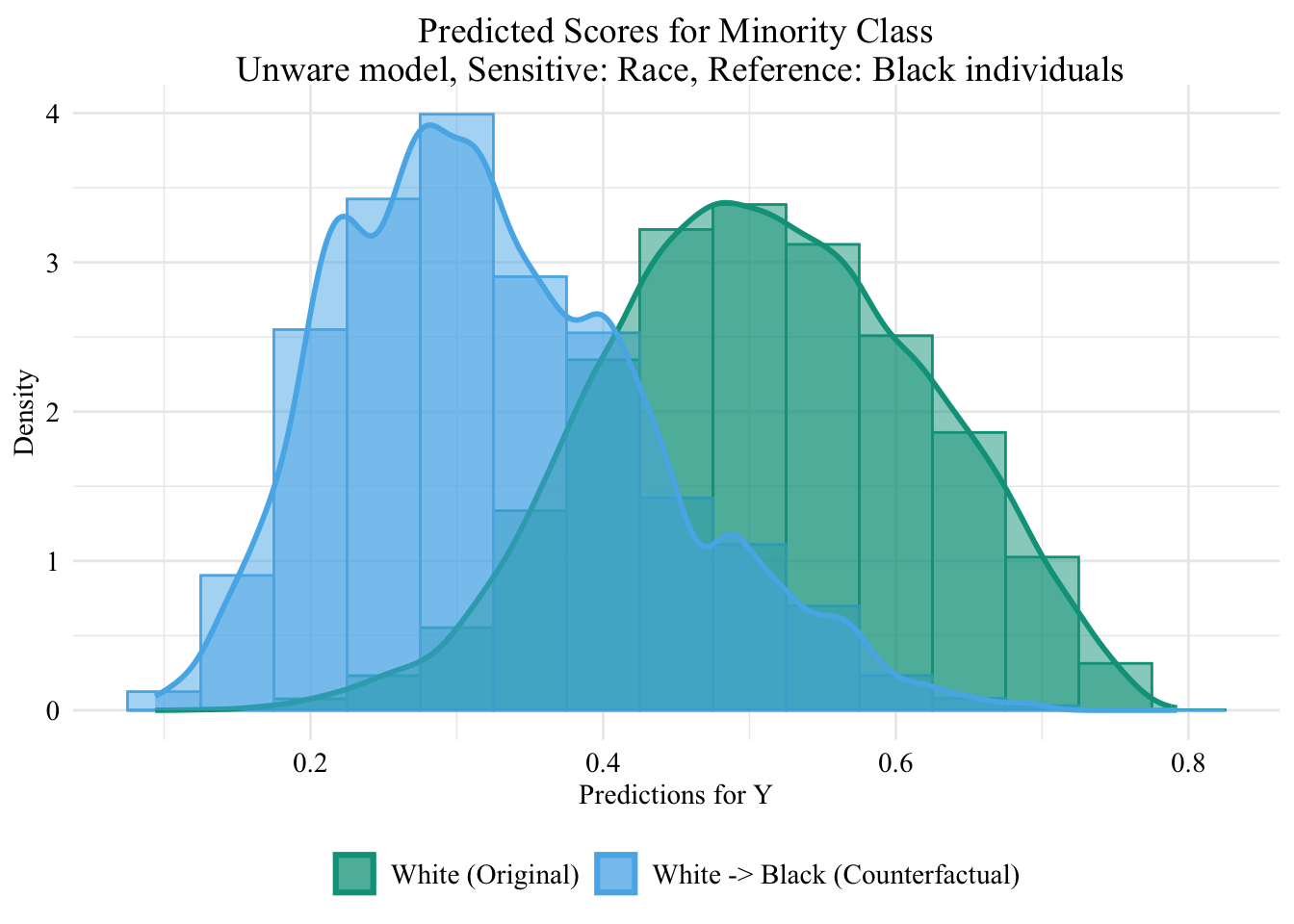
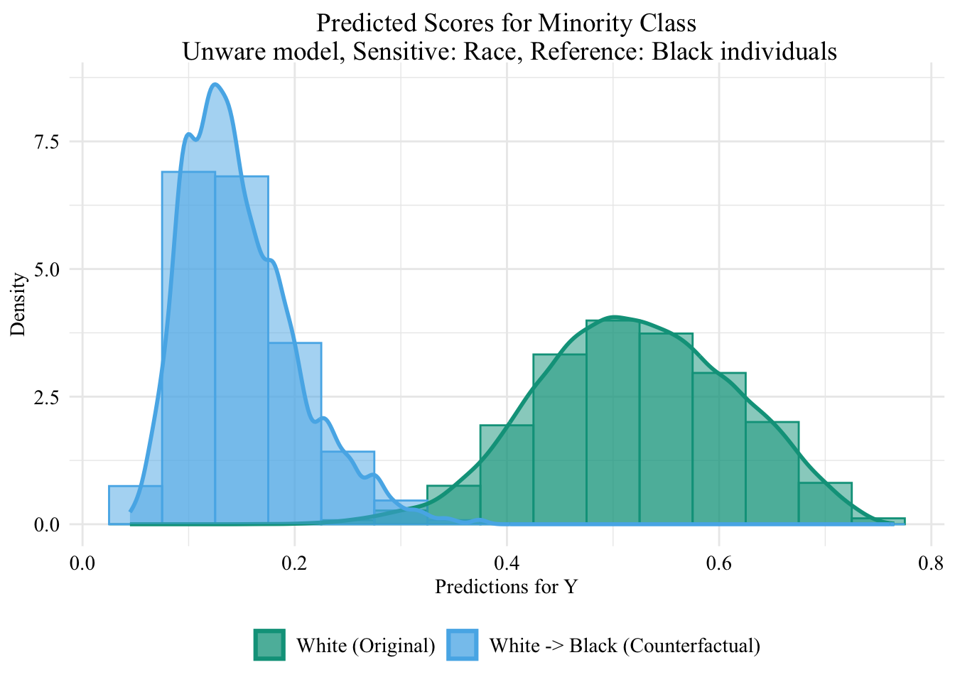
Codes used to create the Figure.
ggplot (data = unaware_ot_white |> mutate (group = case_when (== "White" & S == "White" ~ "White (Original)" ,== "White" & S == "Black" ~ "White -> Black (Counterfactual)" ,== "Black" & S == "Black" ~ "Black (Original)" group = factor (levels = c ("White (Original)" , "White -> Black (Counterfactual)" , "Black (Original)" |> filter (S_origin == "White" ),mapping = aes (x = pred, fill = group, colour = group)+ geom_histogram (mapping = aes (y = after_stat (density)), alpha = 0.5 , position = "identity" , binwidth = 0.05 + geom_density (alpha = 0.5 , linewidth = 1 ) + scale_fill_manual (NULL , values = c ("White (Original)" = colours_all[["source" ]],"White -> Black (Counterfactual)" = colours_all[["ot" ]]+ scale_colour_manual (NULL , values = c ("White (Original)" = colours_all[["source" ]],"White -> Black (Counterfactual)" = colours_all[["ot" ]]+ labs (title = "Predicted Scores for Minority Class \n Unware model, Sensitive: Race, Reference: Black individuals" ,x = "Predictions for Y" ,y = "Density" + global_theme ()
Aware Model
<- tibble (S = df_race_c$ S,S_origin = df_race_c$ S,X1 = df_race_c$ X1,X2 = df_race_c$ X2,Y = df_race_c$ Y,pred = pred_aware_all,type = "factual" |> mutate (id_indiv = row_number ())
We merge the two datasets, factuals_aware and counterfactuals_aware_ot in a single one.
# dataset with counterfactuals, for aware model <- |> mutate (S_origin = S) |> bind_rows (counterfactuals_aware_ot_black)<- |> mutate (S_origin = S) |> bind_rows (counterfactuals_aware_ot_white)
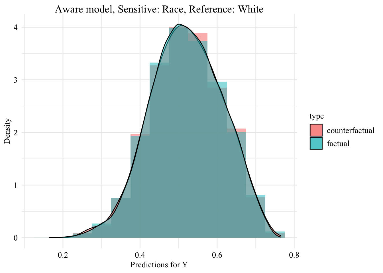
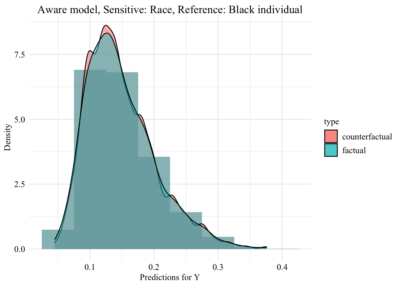
Now, we can visualize the distribution of the values predicted by the unaware model within each group defined by the sensitive attribute.
Codes used to create the Figure.
ggplot (data = aware_ot_black |> mutate (group = case_when (== "Black" & S == "Black" ~ "Black (Original)" ,== "Black" & S == "White" ~ "Black -> White (Counterfactual)" ,== "White" & S == "White" ~ "White (Original)" group = factor (levels = c ("Black (Original)" , "Black -> White (Counterfactual)" , "White (Original)" aes (x = pred, fill = group, colour = group)+ geom_histogram (mapping = aes (y = after_stat (density)), alpha = 0.5 , colour = NA ,position = "identity" , binwidth = 0.05 + geom_density (alpha = 0.3 , linewidth = 1 ) + facet_wrap (~ S) + scale_fill_manual (NULL , values = c ("Black (Original)" = colours_all[["source" ]],"Black -> White (Counterfactual)" = colours_all[["ot" ]],"White (Original)" = colours_all[["reference" ]]+ scale_colour_manual (NULL , values = c ("Black (Original)" = colours_all[["source" ]],"Black -> White (Counterfactual)" = colours_all[["ot" ]],"White (Original)" = colours_all[["reference" ]]+ labs (title = "Aware model, Sensitive: Race, Reference: White individuals" ,x = "Predictions for Y" ,y = "Density" + global_theme () + theme (legend.position = "bottom" )
Codes used to create the Figure.
ggplot (data = aware_ot_white |> mutate (group = case_when (== "White" & S == "White" ~ "White (Original)" ,== "White" & S == "Black" ~ "White -> Black (Counterfactual)" ,== "Black" & S == "Black" ~ "Black (Original)" group = factor (levels = c ("White (Original)" , "White -> Black (Counterfactual)" , "Black (Original)" aes (x = pred, fill = group, colour = group)+ geom_histogram (mapping = aes (y = after_stat (density)), alpha = 0.5 , colour = NA ,position = "identity" , binwidth = 0.05 + geom_density (alpha = 0.3 , linewidth = 1 ) + facet_wrap (~ S) + scale_fill_manual (NULL , values = c ("White (Original)" = colours_all[["source" ]],"White -> Black (Counterfactual)" = colours_all[["ot" ]],"Black (Original)" = colours_all[["reference" ]]+ scale_colour_manual (NULL , values = c ("White (Original)" = colours_all[["source" ]],"White -> Black (Counterfactual)" = colours_all[["ot" ]],"Black (Original)" = colours_all[["reference" ]]+ labs (title = "Aware model, Sensitive: Race, Reference: Black individuals" ,x = "Predictions for Y" ,y = "Density" + global_theme () + theme (legend.position = "bottom" )
Then, we focus on the distribution of predicted scores forcounterfactual of Black students and factuals of white students.
Codes used to create the Figure.
ggplot (data = aware_ot_black |> mutate (group = case_when (== "Black" & S == "Black" ~ "Black (Original)" ,== "Black" & S == "White" ~ "Black -> White (Counterfactual)" ,== "White" & S == "White" ~ "White (Original)" group = factor (levels = c ("Black (Original)" , "Black -> White (Counterfactual)" , "White (Original)" |> filter (S_origin == "Black" ),mapping = aes (x = pred, fill = group, colour = group)+ geom_histogram (mapping = aes (y = after_stat (density)), alpha = 0.5 , position = "identity" , binwidth = 0.05 + geom_density (alpha = 0.5 , linewidth = 1 ) + scale_fill_manual (NULL , values = c ("Black (Original)" = colours_all[["source" ]],"Black -> White (Counterfactual)" = colours_all[["ot" ]],"White (Original)" = colours_all[["reference" ]]+ scale_colour_manual (NULL , values = c ("Black (Original)" = colours_all[["source" ]],"Black -> White (Counterfactual)" = colours_all[["ot" ]],"White (Original)" = colours_all[["reference" ]]+ labs (title = "Predicted Scores for Minority Class \n Unware model, Sensitive: Race, Reference: White individuals" ,x = "Predictions for Y" ,y = "Density" + global_theme ()
Codes used to create the Figure.
ggplot (data = aware_ot_white |> mutate (group = case_when (== "White" & S == "White" ~ "White (Original)" ,== "White" & S == "Black" ~ "White -> Black (Counterfactual)" ,== "Black" & S == "Black" ~ "Black (Original)" group = factor (levels = c ("White (Original)" , "White -> Black (Counterfactual)" , "Black (Original)" |> filter (S_origin == "White" ),mapping = aes (x = pred, fill = group, colour = group)+ geom_histogram (mapping = aes (y = after_stat (density)), alpha = 0.5 , position = "identity" , binwidth = 0.05 + geom_density (alpha = 0.5 , linewidth = 1 ) + scale_fill_manual (NULL , values = c ("White (Original)" = colours_all[["source" ]],"White -> Black (Counterfactual)" = colours_all[["ot" ]]+ scale_colour_manual (NULL , values = c ("White (Original)" = colours_all[["source" ]],"White -> Black (Counterfactual)" = colours_all[["ot" ]]+ labs (title = "Predicted Scores for Minority Class \n Unware model, Sensitive: Race, Reference: Black individuals" ,x = "Predictions for Y" ,y = "Density" + global_theme ()
Saving Objects
save (file = "../data/counterfactuals_unaware_ot_black.rda" save (file = "../data/counterfactuals_aware_ot_black.rda"
De Lara, Lucas, Alberto González-Sanz, Nicholas Asher, Laurent Risser, and Jean-Michel Loubes. 2024. “Transport-Based Counterfactual Models.” Journal of Machine Learning Research 25 (136): 1–59.