7  Classifier

Objectives

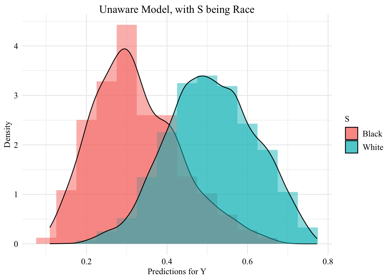
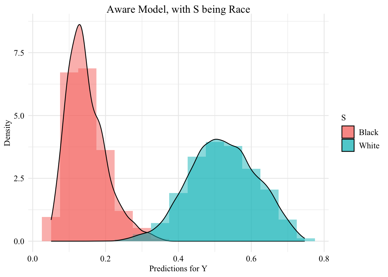
This chapter introduces the scoring classifiers \(m(\cdot)\) trained on the dataset described in Chapter 6. We use logistic regression to predict the outcome \(Y\) based on the covariates \(\boldsymbol{X}\). Two types of models are considered: one that includes the sensitive attribute in the predictive model (aware model) and one that excludes it (unaware model).

# Required packages----
library(tidyverse)

# Graphs----
font_main = font_title = 'Times New Roman'
extrafont::loadfonts(quiet = T)
face_text='plain'
face_title='plain'
size_title = 14
size_text = 11
legend_size = 11

global_theme <- function() {
  theme_minimal() %+replace%
    theme(
      text = element_text(family = font_main, size = size_text, face = face_text),
      legend.text = element_text(family = font_main, size = legend_size),
      axis.text = element_text(size = size_text, face = face_text), 
      plot.title = element_text(
        family = font_title, 
        size = size_title, 
        hjust = 0.5
      ),
      plot.subtitle = element_text(hjust = 0.5),
      legend.position = "bottom"
    )
}

# Seed
set.seed(2025)
colours_all <- c(
  "source" = "#00A08A",
  "reference" = "#F2AD00",
  "naive" = "#000000"
)

Following Kusner et al. (2017), a logistic regression model is trained. To convert \(Y\) into a categorical variable, the median is used as a threshold, in line with Black, Yeom, and Fredrikson (2020). The race, denoted as the sensitive attribute \(S\), has two categories: White and Black. The dataset is divided into training and testing sets. The classifier is first trained and used to compute the necessary quantities for counterfactual inference on the training set. Subsequently, the trained classifier is applied to the test set to make predictions and perform counterfactual analyses. The results of the counterfactuals will also be evaluated on the training set due to the limitation that Optimal Transport in the multivariate case cannot be computed for new samples, unlike the methodologies used in FairAdapt (Plečko, Bennett, and Meinshausen (2021)) and the approach developed in this paper.

7.1 Load Data

We load the data obtained in Chapter 6.3:

load("../data/df_race.rda")

7.2 Pre-processing

First, we transform \(Y\) into a binary variable:

med <- median(df_race$Y)
df_race_c <- df_race |> 
  mutate(
    Y_c = ifelse(Y > med, 1, 0)
  ) |> 
  select(S, X1, X2, Y = Y_c)

We turn the response variable to a factor:

df_race_c$Y <- as.factor(df_race_c$Y)
levels(df_race_c$Y)

[1] "0" "1"

Let us split the dataset into train/test sets (we use the split_dataset() function defined in our small package):

library(devtools)

Loading required package: usethis

load_all("../seqtransfairness/") # load the functions from our package

ℹ Loading seqtransfairness

seed <- 2025
sets <- split_dataset(df_race_c, seed)
data_train <- sets$data_train
data_test <- sets$data_test

7.3 Training the Model

Then, we train two models:

1. unaware logistic regression classifier: model without including the sensitive attribute.
2. aware logistic regression classifier: model with the sensitive attribute included in the set of features.

The model is trained using the log_reg_train() function defined in our small package.

log_reg_train

function(train_data,
                          test_data,
                          s,
                          y,
                          type = c("aware", "unaware")) {
  if (type == "unaware") {
    train_data_ <- train_data |> select(-!!s)
    test_data_ <- test_data |> select(-!!s)
  } else {
    train_data_ <- train_data
    test_data_ <- test_data
  }
  # Train the logistic regression model
  form <- paste0(y, "~.")
  model <- glm(as.formula(form), data = train_data_, family = binomial)
  # Predictions on train and test sets
  pred_train <- predict(model, newdata = train_data_, type = "response")
  pred_test <- predict(model, newdata = test_data_, type = "response")
  list(
    model = model,
    pred_train = pred_train,
    pred_test = pred_test
  )
}
<environment: namespace:seqtransfairness>

Let us train the two models. Then, we extract the predicted values on both the train set and the test set.

# Unaware logistic regression classifier (model without S)
pred_unaware <- log_reg_train(
  data_train, data_test, type = "unaware", s = "S", y = "Y"
)
pred_unaware_train <- pred_unaware$pred_train
pred_unaware_test <- pred_unaware$pred_test

# Aware logistic regression classifier (model with S)
pred_aware <- log_reg_train(
  data_train, data_test, type = "aware", s = "S", y = "Y"
)
pred_aware_train <- pred_aware$pred_train
pred_aware_test <- pred_aware$pred_test

We create a table for each model, with the sensitive attribute and the predicted value by the model (\(\hat{y}\)), only for observations from the test set.

df_test_unaware <- tibble(
  S = data_test$S, 
  pred = pred_unaware_test
)

df_test_aware <- tibble(
  S = data_test$S, 
  pred = pred_aware_test
)

Unaware

ggplot(
  data = df_test_unaware, 
  mapping = aes(x = pred, fill = S)) +
  geom_histogram(
    mapping = aes(y = after_stat(density)), 
    alpha = 0.5, position = "identity", binwidth = 0.05
  ) +
  geom_density(alpha = 0.5) +
  scale_fill_manual(
    "S", values = c(
      "Black" = colours_all[["source"]],
      "White" = colours_all[["reference"]]),
  ) +
  labs(
    title = "Unaware Model, with S being Race",
    x = "Predictions for Y",
    y = "Density"
  ) +
  global_theme()

Figure 7.1: Density of predictions on the test set, for the unaware model, when the sensitive attribute is the race

Aware

ggplot(
  data = df_test_aware,
  mapping = aes(x = pred, fill = S)) +
  geom_histogram(
    mapping = aes(y = after_stat(density)), 
    alpha = 0.5, position = "identity", binwidth = 0.05
  ) +
  geom_density(alpha = 0.5) +
  scale_fill_manual(
    "S", values = c(
      "Black" = colours_all[["source"]],
      "White" = colours_all[["reference"]]),
  ) +
  labs(
    title = "Aware Model, with S being Race",
    x = "Predictions for Y",
    y = "Density"
  ) +
  global_theme()

Figure 7.2: Density of predictions on the test set, for the aware model, when the sensitive attribute is the race

7.4 Predictions

We predict values with the unaware model on the factuals:

model_unaware <- pred_unaware$model
pred_unaware_all <- predict(
  model_unaware, 
  newdata = df_race_c |> select(S, X1, X2), 
  type = "response"
)

And with the aware model:

model_aware <- pred_aware$model
pred_aware_all <- predict(
  model_aware, 
  newdata = df_race_c |> select(S, X1, X2), 
  type = "response"
)

7.5 Saving Objects

save(df_race_c, file = "../data/df_race_c.rda")
save(pred_aware, file = "../data/pred_aware.rda")
save(pred_unaware, file = "../data/pred_unaware.rda")
save(pred_unaware_all, file = "../data/pred_unaware_all.rda")
save(pred_aware_all, file = "../data/pred_aware_all.rda")

Black, Emily, Samuel Yeom, and Matt Fredrikson. 2020. “Fliptest: Fairness Testing via Optimal Transport.” In Proceedings of the 2020 Conference on Fairness, Accountability, and Transparency, 111–21.

Kusner, Matt J, Joshua Loftus, Chris Russell, and Ricardo Silva. 2017. “Counterfactual Fairness.” In Advances in Neural Information Processing Systems 30, edited by I. Guyon, U. V. Luxburg, S. Bengio, H. Wallach, R. Fergus, S. Vishwanathan, and R. Garnett, 4066–76. NIPS.

Plečko, Drago, Nicolas Bennett, and Nicolai Meinshausen. 2021. “Fairadapt: Causal Reasoning for Fair Data Pre-Processing.” arXiv Preprint arXiv:2110.10200.