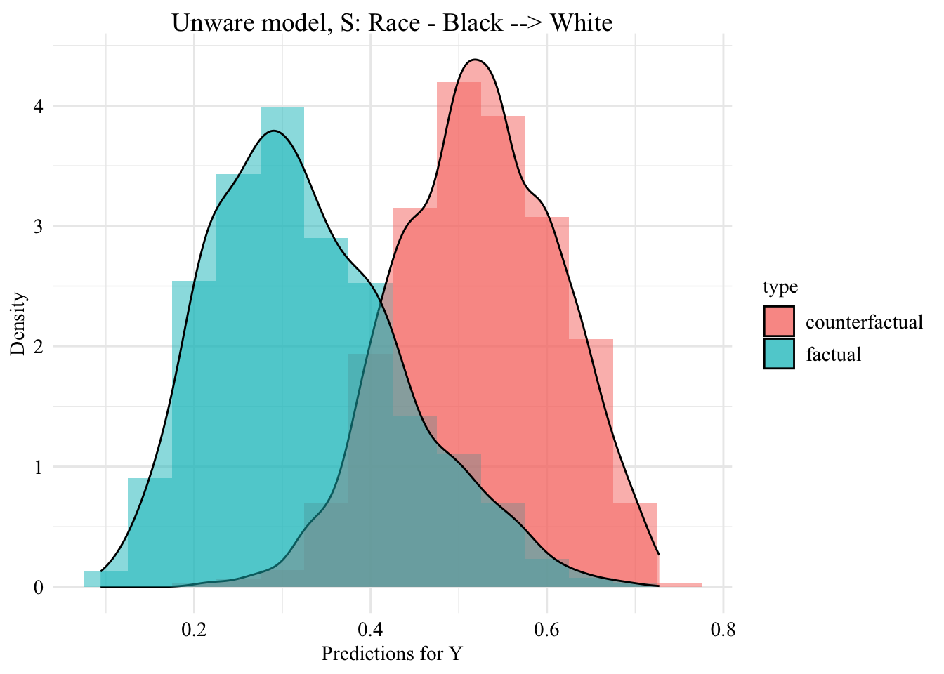
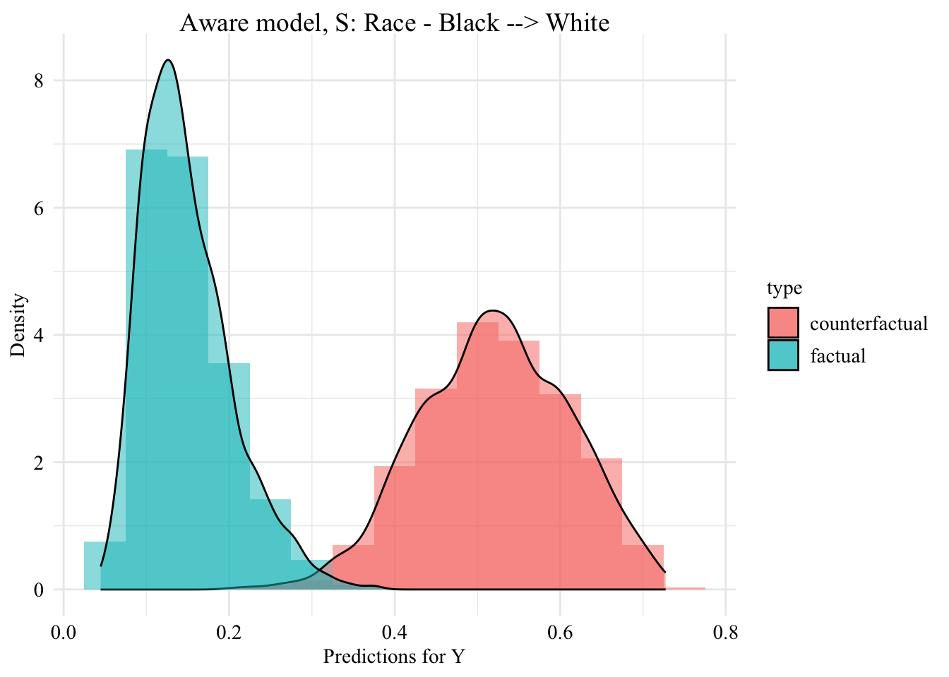
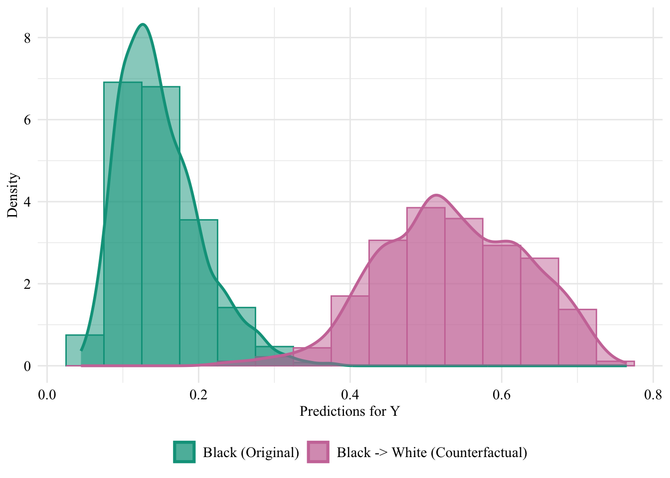
This chapter uses sequential transport (methodology developped in our paper) to make counterfactual inference. We obtain counterfactual values \(\boldsymbol{x}^\star\) for individuals from the protected group \(S=0\). Then, we use the aware and unaware classifiers \(m(\cdot)\) (see Chapter 7) to make new predictions \(m(s=1,\boldsymbol{x}^\star)\) for individuals in the protected class, i.e., observations in \(\mathcal{D}_0\).
In the article, we use three methods to create counterfactuals:
We load the dataset where the sensitive attribute (\(S\)) is the race, obtained Chapter 6.3:
load("../data/df_race.rda")
We also load the dataset where the sensitive attribute is also the race, but where where the target variable (\(Y\), ZFYA) is binary (1 if the student obtained a standardized first year average over the median, 0 otherwise). This dataset was saved in Chapter 7.5:
load("../data/df_race_c.rda")
We also need the predictions made by the classifier (see Chapter 7):
# Predictions on train/test setsload("../data/pred_aware.rda")load("../data/pred_unaware.rda")# Predictions on the factuals, on the whole datasetload("../data/pred_aware_all.rda")load("../data/pred_unaware_all.rda")
11.2 Counterfactuals with Sequential Transport
We now turn to sequential transport (the methodology developed in our paper). We define a function, seq_trans() (see in functions/utils.R) to perform a fast sequential transport on causal graph.
R codes for functions seq_trans(), topological_ordering(), and swap()
#' Sequential Transport Using a Pre-Defined Causal Graph#'#' The sensitive attribute, S, is assumed to be a binary variable with value#' $S_0$ in the source distribution and $S_1$ in the target distribution.#'#' @param data Data frame with the observations.#' @param adj Adjacency matrix for the causal graph.#' @param s Name of the sensitive attribute column in the data.#' @param S_0 Label of the sensitive attribute in the source distribution.#' @param y Name of the outcome variable in the data.#' @param num_neighbors Number of neighbors to use in the weighted quantile#' estimation. Default to 5.#' @param silent If `TRUE`, the messages showing progress in the estimation are#' not shown. Default to `silent=FALSE`.#'#' @returns A list with the following elements:#' * `transported`: A named list with the transported values. The names are those of the variables.#' * `weights`: A list with the weights of each observation in the two groups.#' * `ecdf`: A list with empirical distribution functions for numerical variables.#' * `ecdf_values`: A list with the values of the ecdf evaluated for each observation in the source distribution.#' * `fit_for_categ`: A list with the estimated multinomial models to predict categories using parents characteristics#' * `params`: A list with some parameters used to transport observations:#' * `adj`: Adjacency matrix.#' * `top_order`: Topological ordering.#' * `s`: Name of the sensitive attribute.#' * `S_0`: Label of the sensitive attribute in the source distribution.#' * `y`: Name of the outcome variable in the data.#' * `num_neighbors`: Number of neighbors used when computing quantiles.#' @md#' @export#'#' @importFrom stats predict ecdf quantile#' @importFrom dplyr across filter mutate pull select#' @importFrom tidyselect where#' @importFrom rlang sym !! := is_character#' @importFrom cluster daisy#' @importFrom Hmisc wtd.quantile#' @importFrom nnet multinomseq_trans <-function(data, adj, s, S_0, y,num_neighbors =5,silent =FALSE) {# Make sure character variables are encoded as factors data <- data |>mutate(across(where(is_character), ~as.factor(.x)))# Topological ordering top_order <-topological_ordering(adj) variables <- top_order[!top_order %in%c(s, y)]# Observations in group S_0 data_0 <- data |>filter(!!sym(s) ==!!S_0) data_1 <- data |>filter(!!sym(s) !=!!S_0)# Lists where results will be stored list_transported <-list() # Transported values list_weights <-list() # Weights list_ecdf <-list() # Empirical dist. function list_ecdf_values <-list() # Evaluated values of the ecdf fit_for_categ <-list() # Fitted multinomial models for categ. variablesfor (x_name in variables) {if (silent ==FALSE) cat("Transporting ", x_name, "\n")# Names of the parent variables parents <-colnames(adj)[adj[, x_name] ==1]# values of current x in each group x_S0 <- data_0 |>pull(!!x_name) x_S1 <- data_1 |>pull(!!x_name)# Check whether X is numeric is_x_num <-is.numeric(x_S0)# Characteristics of the parent variables (if any) parents_characteristics <- data_0 |>select(!!parents) |>select(-!!s)if (length(parents_characteristics) >0) { data_0_parents <- data_0 |>select(!!parents) |>select(-!!s) data_1_parents <- data_1 |>select(!!parents) |>select(-!!s)# Weights in S_0 weights_S0 <-as.matrix(cluster::daisy(data_0_parents, metric ="gower")) tot_weights_S0 <-apply(weights_S0, MARGIN =1, sum)# Weights in S_1# First, we need to get the transported values for the parents, if necessary data_0_parents_t <- data_0_parents #initfor (parent in parents) {# does the parent depend on the sensitive variableif (parent %in%names(list_transported)) { data_0_parents_t <- data_0_parents_t |>mutate(!!sym(parent) := list_transported[[parent]]) } }# Unfortunately, we will compute a lot of distances not needed combined <-rbind(data_0_parents_t, data_1_parents) gower_dist <- cluster::daisy(combined, metric ="gower") gower_matrix <-as.matrix(gower_dist) n_0 <-nrow(data_0_parents_t) n_1 <-nrow(data_1_parents) weights_S1 <- gower_matrix[1:n_0, (n_0 +1):(n_0 + n_1), drop =FALSE] weights_S1 <- weights_S1 +1e-8 weights_S1 <-1/ (weights_S1)^2 tot_weights_S1 <-apply(weights_S1, MARGIN =1, sum)if (is_x_num ==TRUE) {# Numerical variable to transport# Empirical distribution function f <-rep(NA, length(x_S0))for (i in1:length(x_S0)) { f[i] <- weights_S0[i, ] %*% (x_S0 <= x_S0[i]) / tot_weights_S0[i] } list_ecdf_values[[x_name]] <- f f[f==1] <-1-(1e-8)# Transported values transported <-rep(NA, length(x_S0))for (i in1:length(x_S0)) { wts <- weights_S1[i, ] wts[-order(wts, decreasing =TRUE)[1:num_neighbors]] <-0 transported[i] <- Hmisc::wtd.quantile(x = x_S1, weights = weights_S1[i, ], probs = f[i] ) |>suppressWarnings() } } else {# X is non numeric and has parents# Fit a model to predict the categorical variables given the# characteristics of the parents in group to transport into fit_indix_x <- nnet::multinom( x_S0 ~ .,data = data_1_parents |>mutate(x_S0 = x_S1) )# Predictions with that model for transported parents pred_probs <-predict(fit_indix_x, type ="probs", newdata = data_0_parents_t)# For each observation, random draw of the class, using the pred probs# as weights drawn_class <-apply( pred_probs, 1,function(x) sample(1:ncol(pred_probs), prob = x, size =1) ) transported <-colnames(pred_probs)[drawn_class]if (is.factor(x_S1)) { transported <-factor(transported, levels =levels(x_S1)) } fit_for_categ[[x_name]] <- fit_indix_x } list_transported[[x_name]] <- transported# Store weights for possible later use list_weights[[x_name]] <-list(w_S0 =list(weights = weights_S0, tot_weights = tot_weights_S0),w_S1 =list(weights = weights_S1, tot_weights = tot_weights_S1) ) } else {# No parentsif (is_x_num ==TRUE) {# X is numerical and has no parents F_X_S0 <-ecdf(x_S0) list_ecdf[[x_name]] <- F_X_S0 f <-F_X_S0(x_S0) list_ecdf_values[[x_name]] <- f transported <-as.numeric(quantile(x_S1, probs = f)) } else {# X is not numerical and has no parents transported <-sample(x_S1, size =length(x_S0), replace =TRUE)if (is.factor(x_S1)) { transported <-factor(transported, levels =levels(x_S1)) } else { transported <-as.factor(transported) } } list_transported[[x_name]] <- transported } }return(list(transported = list_transported,weights = list_weights,ecdf = list_ecdf,ecdf_values = list_ecdf_values,fit_for_categ = fit_for_categ,params =list(adj = adj,top_order = top_order,s = s,S_0 = S_0,y = y,num_neighbors = num_neighbors ) ) )}#' Topological Ordering#'#' @source This function comes from the fairadapt package. Drago Plecko,#' Nicolai Meinshausen (2020). Fair data adaptation with quantile#' preservation Journal of Machine Learning Research, 21.242, 1-44.#' URL https://www.jmlr.org/papers/v21/19-966.html.#' @param adj_mat Adjacency matrix with names of the variables for both rows and#' columns.#' @return A character vector (names of the variables) providing a topological#' ordering.#' @exporttopological_ordering <-function(adj_mat) { nrw <-nrow(adj_mat) num_walks <- adj_matfor (i inseq_len(nrw +1L)) { num_walks <- adj_mat + num_walks %*% adj_mat } comparison_matrix <- num_walks >0 top_order <-colnames(adj_mat)for (i inseq_len(nrw -1L)) {for (j inseq.int(i +1L, nrw)) {if (comparison_matrix[top_order[j], top_order[i]]) { top_order <-swap(top_order, i, j) } } } top_order}#' Swap Two Elements in a Matrix.#'#' @source This function comes from the fairadapt package. Drago Plecko,#' Nicolai Meinshausen (2020). Fair data adaptation with quantile#' preservation Journal of Machine Learning Research, 21.242, 1-44.#' URL https://www.jmlr.org/papers/v21/19-966.html.#' @param x A matrix.#' @param i Index of the first element to swap.#' @param j Index of the second element to swap.#' @return The matrix x where the i-th and j-th elements have been swapped.#' @noRdswap <-function(x, i, j) { keep <- x[i] x[i] <- x[j] x[j] <- keep x}
Let us apply this function, but first, we create a dataset, df_race_c_light, with the sensitive attribute and the two characteristics only:
We first transport \(x_1\), then \(x_2\), assuming that \(x_1\) is influenced by \(S\) only, \(x_2\) is influenced by both \(S\) and \(x_1\), and \(Y\) is influenced by \(S\), \(x_1\), and \(x_2\).
x1_star <- trans_x1_then_x2$transported$X1 # Transport X1 to group S=Whitex2_star <- trans_x1_then_x2$transported$X2 # Transport X2|X1 to group S=White
We build a dataset with the sensitive attribute of Black individuals changed to white, and their characteristics changed to their transported characteristics:
Let us put in a single table the predictions made by the classifier (either aware or unaware) on Black and White individuals based on their factual characteristics, and those made based on the counterfactuals (i.e., only for Black individuals).